Curriculum for Reinforcement Learning
Curriculum for Reinforcement Learning.
- Task-Specific Curriculum
- Teacher-Guided Curriculum
- Curriculum through Self-Play
- Automatic Goal Generation
- Skill-Based Curriculum
It sounds like an impossible task if we want to teach integral or derivative to a 3-year-old who does not even know basic arithmetics. That’s why education is important, as it provides a systematic way to break down complex knowledge and a nice curriculum for teaching concepts from simple to hard. A curriculum makes learning difficult things easier and approachable for us humans. But, how about machine learning models? Can we train our models more efficiently with a curriculum? Can we design a curriculum to speed up learning?
Back in 1993, Jeffrey Elman has proposed the idea of training neural networks with a curriculum. His early work on learning simple language grammar demonstrated the importance of such a strategy: starting with a restricted set of simple data and gradually increasing the complexity of training samples; otherwise the model was not able to learn at all.
Compared to training without a curriculum, we would expect the adoption of the curriculum to expedite the speed of convergence and may or may not improve the final model performance. To design an efficient and effective curriculum is not easy. Keep in mind that, a bad curriculum may even hamper learning.
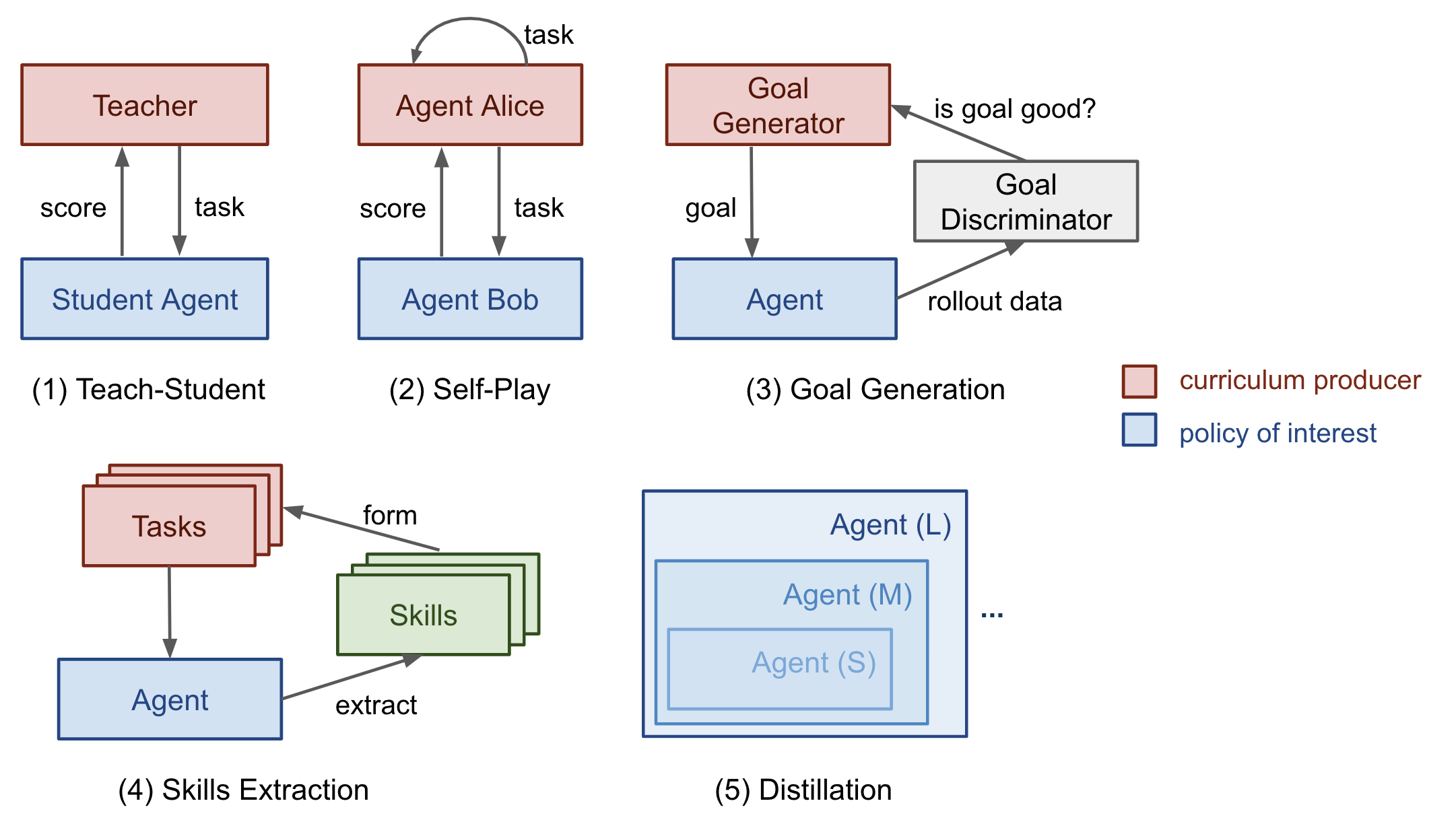
Next, we will look into several categories of curriculum learning, as illustrated in Fig. 1. Most cases are applied to Reinforcement Learning, with a few exceptions on Supervised Learning.
In “The importance of starting small” paper (Elman 1993), I especially like the starting sentences and find them both inspiring and affecting:
“Humans differ from other species along many dimensions, but two are particularly noteworthy. Humans display an exceptional capacity to learn; and humans are remarkable for the unusually long time it takes to reach maturity. The adaptive advantage of learning is clear, and it may be argued that, through culture, learning has created the basis for a non-genetically based transmission of behaviors which may accelerate the evolution of our species”
Indeed, learning is probably the best superpower we humans have.
Task-Specific Curriculum
Bengio, et al. (2009) provided a good overview of curriculum learning in the old days. The paper presented two ideas with toy experiments using a manually designed task-specific curriculum:
- Cleaner Examples may yield better generalization faster.
- Introducing gradually more difficult examples speeds up online training.
It is plausible that some curriculum strategies could be useless or even harmful. A good question to answer in the field is: What could be the general principles that make some curriculum strategies work better than others? The Bengio 2009 paper hypothesized it would be beneficial to make learning focus on “interesting” examples that are neither too hard or too easy.
If our naive curriculum is to train the model on samples with a gradually increasing level of complexity, we need a way to quantify the difficulty of a task first. One idea is to use its minimal loss with respect to another model while this model is pretrained on other tasks (Weinshall, et al. 2018). In this way, the knowledge of the pretrained model can be transferred to the new model by suggesting a rank of training samples. Fig. 2 shows the effectiveness of the curriculum group (green), compared to control (random order; yellow) and anti (reverse the order; red) groups.
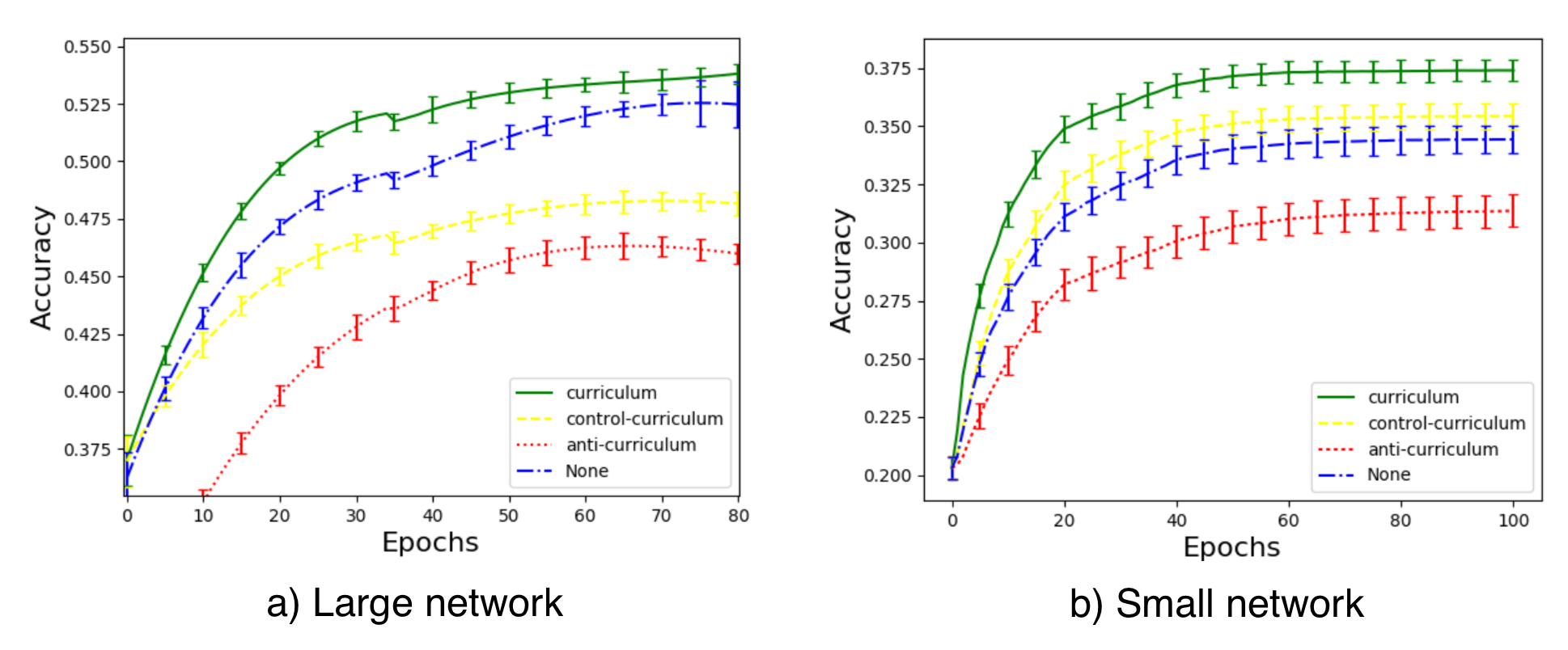 Fig. 2. Image classification accuracy on test image set (5 member classes of “small mammals” in CIFAR100). There are 4 experimental groups, (a)
 curriculum: sort the labels by the confidence of another trained classifier (e.g. the margin of an SVM); (b) control-curriculum: sort the labels randomly; (c) anti-curriculum: sort the labels reversely; (d) None: no curriculum. (Image source: Weinshall, et al. 2018)
Zaremba and Sutskever (2014) did an interesting experiment on training LSTM to predict the output of a short Python program for mathematical ops without actually executing the code. They found curriculum is necessary for learning. The program’s complexity is controlled by two parameters, length ∈ [1, a] and nesting∈ [1, b]. Three strategies are considered:
- Naive curriculum: increase
lengthfirst until reachinga; then increasenestingand resetlengthto 1; repeat this process until both reach maximum. - Mix curriculum: sample
length~ [1, a] andnesting~ [1, b] - Combined: naive + mix.
They noticed that combined strategy always outperformed the naive curriculum and would generally (but not always) outperform the mix strategy — indicating that it is quite important to mix in easy tasks during training to avoid forgetting. Procedural content generation (PCG) is a popular approach for creating video games of various levels of difficulty. PCG involves algorithmic randomness and a heavy dose of human expertise in designing game elements and dependencies among them. Procedurally generated levels have been introduced into several benchmark environments for evaluating whether an RL agent can generalize to a new level that it is not trained on (meta-RL), such as GVGAI, OpenAI CoinRun and Procgen benchmark. Using GVGAI, Justesen, et al. (2018) demonstrated that an RL policy can easily overfit to a specific game but training over a simple curriculum that grows the task difficulty together with the model performance helps its generalization to new human-designed levels. Similar results are also found in CoinRun (Cobbe, et al. 2018). POET (Wang et al, 2019) is another example for leveraging evolutionary algorithm and procedural generated game levels to improve RL generalization, which I’ve described in details in my meta-RL post To follow the curriculum learning approaches described above, generally we need to figure out two problems in the training procedure:
- Design a metric to quantify how hard a task is so that we can sort tasks accordingly.
- Provide a sequence of tasks with an increasing level of difficulty to the model during training.
However, the order of tasks does not have to be sequential. In our Rubik’s cube paper (OpenAI et al, 2019), we depended on Automatic domain randomization (ADR) to generate a curriculum by growing a distribution of environments with increasing complexity. The difficulty of each task (i.e. solving a Rubik’s cube in a set of environments) depends on the randomization ranges of various environmental parameters. Even with a simplified assumption that all the environmental parameters are uncorrelated, we were able to create a decent curriculum for our robot hand to learn the task.
Teacher-Guided Curriculum
The idea of Automatic Curriculum Learning was proposed by Graves, et al. 2017 slightly earlier. It considers a N-task curriculum as an N-armed bandit problem and an adaptive policy which learns to optimize the returns from this bandit. Two categories of learning signals have been considered in the paper:
- Loss-driven progress: the loss function change before and after one gradient update. This type of reward signals tracks the speed of the learning process, because the greatest task loss decrease is equivalent to the fastest learning.
- Complex-driven progress: the KL divergence between posterior and prior distribution over network weights. This type of learning signals are inspired by the MDL principle, increasing the model complexity by a certain amount is only worthwhile if it compresses the data by a greater amount. The model complexity is therefore expected to increase most in response to the model nicely generalizing to training examples.
This framework of proposing curriculum automatically through another RL agent was formalized as Teacher-Student Curriculum Learning (TSCL; Matiisen, et al. 2017). In TSCL, a student is an RL agent working on actual tasks while a teacher agent is a policy for selecting tasks. The student aims to master a complex task that might be hard to learn directly. To make this task easier to learn, we set up the teacher agent to guide the student’s training process by picking proper sub-tasks.
 Fig. 3. The setup of teacher-student curriculum learning. (Image source: Matiisen, et al. 2017 + my annotation in red.)
In the process, the student should learn tasks which:
- can help the student make fastest learning progress, or
- are at risk of being forgotten.
Note: The setup of framing the teacher model as an RL problem feels quite similar to Neural Architecture Search (NAS), but differently the RL model in TSCL operates on the task space and NAS operates on the main model architecture space.
Training the teacher model is to solve a POMDP problem:
- The unobserved $s_t$ is the full state of the student model.
- The observed $o = (x_t^{(1)}, \dots, x_t^{(N)})$ are a list of scores for $N$ tasks.
- The action $a$ is to pick on subtask.
- The reward per step is the score delta $r_{t} = \sum_{i=1}^{N} x_t^{(i)} - x_{t-1}^{(i)}$ (i.e., equivalent to maximizing the score of all tasks at the end of the episode).
The method of estimating learning progress from noisy task scores while balancing exploration vs exploitation can be borrowed from the non-stationary multi-armed bandit problem - use ε-greedy, or Thompson sampling.
The core idea, in summary, is to use one policy to propose tasks for another policy to learn better. Interestingly, both works above (in the discrete task space) found that uniformly sampling from all tasks is a surprisingly strong benchmark.
What if the task space is continuous? Portelas, et al. (2019) studied a continuous teacher-student framework, where the teacher has to sample parameters from continuous task space to generate a learning curriculum. Given a newly sampled parameter $p$, the absolute learning progress (short for ALP) is measured as $\text{ALP}_p = \vert r - r_\text{old} \vert $, where $r$ is the episodic reward associated with $p$ and $r_\text{old}$ is the reward associated with $p_\text{old}$. Here, $p_\text{old}$ is a previous sampled parameter closest to $p$ in the task space, which can be retrieved by nearest neighbor. Note that how this ALP score is different from learning signals in TSCL or Grave, et al. 2017 above: ALP score measures the reward difference between two tasks rather than performance at two time steps of the same task.
On top of the task parameter space, a Gaussian mixture model is trained to fit the distribution of $ \text{ALP}_p $ over $p$. ε-greedy is used when sampling the tasks: with some probability, sampling a random task; otherwise sampling proportionally to ALP score from the GMM model.
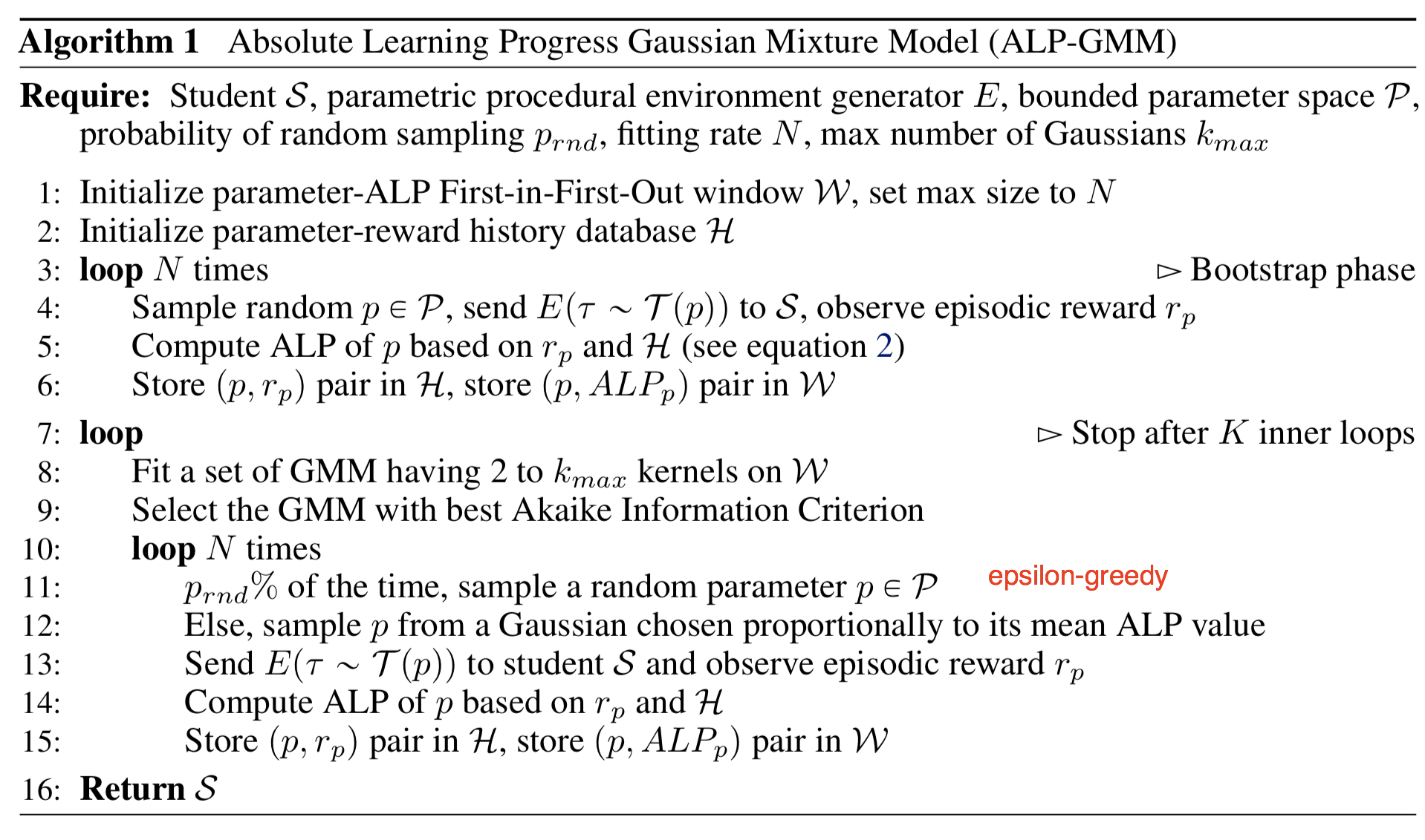 Fig. 4. The algorithm of ALP-GMM (absolute learning progress Gaussian mixture model). (Image source: Portelas, et al., 2019)
Curriculum through Self-Play
Different from the teacher-student framework, two agents are doing very different things. The teacher learns to pick a task for the student without any knowledge of the actual task content. What if we want to make both train on the main task directly? How about even make them compete with each other?
Sukhbaatar, et al. (2017) proposed a framework for automatic curriculum learning through asymmetric self-play. Two agents, Alice and Bob, play the same task with different goals: Alice challenges Bob to achieve the same state and Bob attempts to complete it as fast as he can.
 Fig. 5. Illustration of the self-play setup when training two agents. The example task is MazeBase: An agent is asked to reach a goal flag in a maze with a light switch, a key and a wall with a door. Toggling the key switch can open or close the door and Turning off the light makes only the glowing light switch available to the agent. (Image source: Sukhbaatar, et al. 2017)
Let us consider Alice and Bob as two separate copies for one RL agent trained in the same environment but with different brains. Each of them has independent parameters and loss objective. The self-play-driven training consists of two types of episodes:
- In the
self-play episode, Alice alters the state from $s_0$ to $s_t$ and then Bob is asked to return the environment to its original state $s_0$ to get an internal reward. - In the
target task episode, Bob receives an external reward if he visits the target flag.
Note that since B has to repeat the actions between the same pair of $(s_0, s_t)$ of A, this framework only works in reversible or resettable environments. Alice should learn to push Bob out of his comfort zone, but not give him impossible tasks. Bob’s reward is set as $R_B = -\gamma t_B$ and Alice’s reward is $R_A = \gamma \max(0, t_B - t_A)$, where $t_B$ is the total time for B to complete the task, $t_A$ is the time until Alice performs the STOP action and $\gamma$ is a scalar constant to rescale the reward to be comparable with the external task reward. If B fails a task, $t_B = t_\max - t_A$. Both policies are goal-conditioned. The losses imply:
- B wants to finish a task asap.
- A prefers tasks that take more time of B.
- A does not want to take too many steps when B is failing.
In this way, the interaction between Alice and Bob automatically builds a curriculum of increasingly challenging tasks. Meanwhile, as A has done the task herself before proposing the task to B, the task is guaranteed to be solvable. The paradigm of A suggesting tasks and then B solving them does sound similar to the Teacher-Student framework. However, in asymmetric self-play, Alice, who plays a teacher role, also works on the same task to find challenging cases for Bob, rather than optimizes B’s learning process explicitly.
Automatic Goal Generation
Often RL policy needs to be able to perform over a set of tasks. The goal should be carefully chosen so that at every training stage, it would not be too hard or too easy for the current policy. A goal $g \in \mathcal{G}$ can be defined as a set of states $S^g$ and a goal is considered as achieved whenever an agent arrives at any of those states. The approach of Generative Goal Learning (Florensa, et al. 2018) relies on a Goal GAN to generate desired goals automatically. In their experiment, the reward is very sparse, just a binary flag for whether a goal is achieved or not and the policy is conditioned on goal,
Here $R^g(\pi)$ is the expected return, also equivalent to the success probability. Given sampled trajectories from the current policy, as long as any state belongs to the goal set, the return will be positive. Their approach iterates through 3 steps until the policy converges:
-
Label a set of goals based on whether they are at the appropriate level of difficulty for the current policy.
- The set of goals at the appropriate level of difficulty are named GOID (short for “Goals of Intermediate Difficulty”) $\text{GOID}_i := {g : R_\text{min} \leq R^g(\pi_i) \leq R_\text{max} } \subseteq G$
-
Here $R_\text{min}$ and $R_\text{max}$ can be interpreted as a minimum and maximum probability of reaching a goal over T time-steps.
- Train a Goal GAN model using labelled goals from step 1 to produce new goals
- Use these new goals to train the policy, improving its coverage objective.
The Goal GAN generates a curriculum automatically:
- Generator $G(z)$: produces a new goal. => expected to be a goal uniformly sampled from $GOID$ set.
- Discriminator $D(g)$: evaluates whether a goal can be achieved. => expected to tell whether a goal is from $GOID$ set.
The Goal GAN is constructed similar to LSGAN (Least-Squared GAN; Mao et al., (2017)), which has better stability of learning compared to vanilla GAN. According to LSGAN, we should minimize the following losses for $D$ and $G$ respectively:
where $a$ is the label for fake data, $b$ for real data, and $c$ is the value that $G$ wants $D$ to believe for fake data. In LSGAN paper’s experiments, they used $a=-1, b=1, c=0$. The Goal GAN introduces an extra binary flag $y_b$ indicating whether a goal $g$ is real ($y_{g} = 1$) or fake ($y_{g} = 0$) so that the model can use negative samples for training:
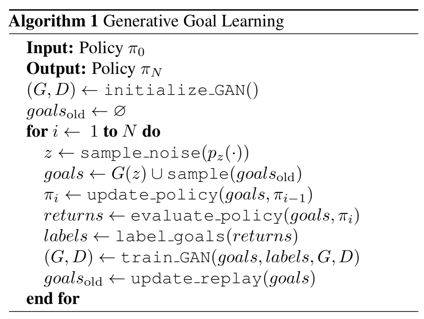 Fig. 6. The algorithm of Generative Goal Learning. (Image source: (Florensa, et al. 2018)
Following the same idea, Racaniere and Lampinen, et al. (2019) designs a method to make the objectives of goal generator more sophisticated. Their method contains three components, same as generative goal learning above:
- Solver /Policy $\pi$: In each episode, the solver gets a goal $g$ at the beginning and get a single binary reward $R^g$ at the end.
- Judge /Discriminator $D(.)$: A classifier to predict the binary reward (whether goal can be achieved or not); precisely it outputs the logit of a probability of achieving the given goal, $\sigma(D(g)) = p(R^g=1\vert g)$, where $\sigma$ is the sigmoid function.
- Setter /Generator $G(.)$: The goal setter takes as input a desired feasibility score $f \in \text{Unif}(0, 1)$ and generates $g = G(z, f)$, where the latent variable $z$ is sampled by $z \sim \mathcal{N}(0, I)$. The goal generator is designed to reversible, so $G^{-1}$ can map backwards from a goal $g$ to a latent $z = G^{-1}(g, f)$
The generator is optimized with three objectives:
Goal validity: The proposed goal should be achievable by an expert policy. The corresponding generative loss is designed to increase the likelihood of generating goals that the solver policy has achieved before (like in HER).
$\mathcal{L}_\text{val}$ is the negative log-likelihood of generated goals that have been solved by the solver in the past.
Goal feasibility: The proposed goal should be achievable by the current policy; that is, the level of difficulty should be appropriate.
$\mathcal{L}_\text{feas}$ is the output probability by the judge model $D$ on the generated goal $G(z, f)$ should match the desired $f$.
- Goal coverage: We should maximize the entropy of generated goals to encourage diverse goal and to improve the coverage over the goal space.
Their experiments showed complex environments require all three losses above. When the environment is changing between episodes, both the goal generator and the discriminator need to be conditioned on environmental observation to produce better results. If there is a desired goal distribution, an additional loss can be added to match a desired goal distribution using Wasserstein distance. Using this loss, the generator can push the solver toward mastering the desired tasks more efficiently.
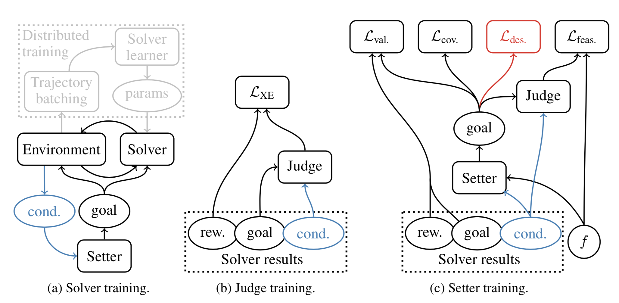 Fig. 7. Training schematic for the (a) solver/policy, (b) judge/discriminator, and (c) setter/goal generator models. (Image source: Racaniere & Lampinen, et al., 2019)
Skill-Based Curriculum
Another view is to decompose what an agent is able to complete into a variety of skills and each skill set could be mapped into a task. Let’s imagine when an agent interacts with the environment in an unsupervised manner, is there a way to discover useful skills from such interaction and further build into the solutions for more complicated tasks through a curriculum?
Jabri, et al. (2019) developed an automatic curriculum, CARML (short for “Curricula for Unsupervised Meta-Reinforcement Learning”), by modeling unsupervised trajectories into a latent skill space, with a focus on training meta-RL( policies (i.e. can transfer to unseen tasks). The setting of training environments in CARML is similar to DIAYN. Differently, CARML is trained on pixel-level observations but DIAYN operates on the true state space. An RL algorithm $\pi_\theta$, parameterized by $\theta$, is trained via unsupervised interaction formulated as a CMP combined with a learned reward function $r$. This setting naturally works for the meta-learning purpose, since a customized reward function can be given only at the test time.
 Fig. 8. An illustration of CARML, containing two steps: (1) organizing experiential data into the latent skill space; (2) meta-training the policy with the reward function constructed from the learned skills. (Image source: Jabri, et al 2019)
CARML is framed as a variational Expectation-Maximization (EM).
(1) E-Step: This is the stage for organizing experiential data. Collected trajectories are modeled with a mixture of latent components forming the basis of skills.
Let $z$ be a latent task variable and $q_\phi$ be a variational distribution of $z$, which could be a mixture model with discrete $z$ or a VAE with continuous $z$. A variational posterior $q_\phi(z \vert s)$ works like a classifier, predicting a skill given a state, and we would like to maximize $q_\phi(z \vert s)$ to discriminate between data produced by different skills as much as possible. In E-step, $q_\phi$ is fitted to a set of trajectories produced by $\pi_\theta$.
Precisely, given a trajectory $\tau = (s_1,\dots,s_T)$, we would like to find $\phi$ such that
A simplifying assumption is made here to ignore the order of states in one trajectory. (2) M-Step: This is the stage for doing meta-RL training with $\pi_\theta$. The learned skill space is considered as a training task distribution. CARML is agnostic to the type of meta-RL algorithm for policy parameter updates. Given a trajectory $\tau$, it makes sense for the policy to maximize the mutual information between $\tau$ and $z$, $I(\tau;z) = H(\tau) - H(\tau \vert z)$, because:
- maximizing $H(\tau)$ => diversity in the policy data space; expected to be large.
- minimizing $H(\tau \vert z)$ => given a certain skill, the behavior should be restricted; expected to be small.
Then we have,
We can set the reward as $\log q_\phi(s \vert z) - \log q_\phi(s)$, as shown in the green part in the equation above. In order to balance between task-specific exploration (as in red below) and latent skill matching (as in blue below) , a parameter $\lambda \in [0, 1]$ is added. Each realization of $z \sim q_\phi(z)$ induces a reward function $r_z(s)$ (remember that reward + CMP => MDP) as follows:
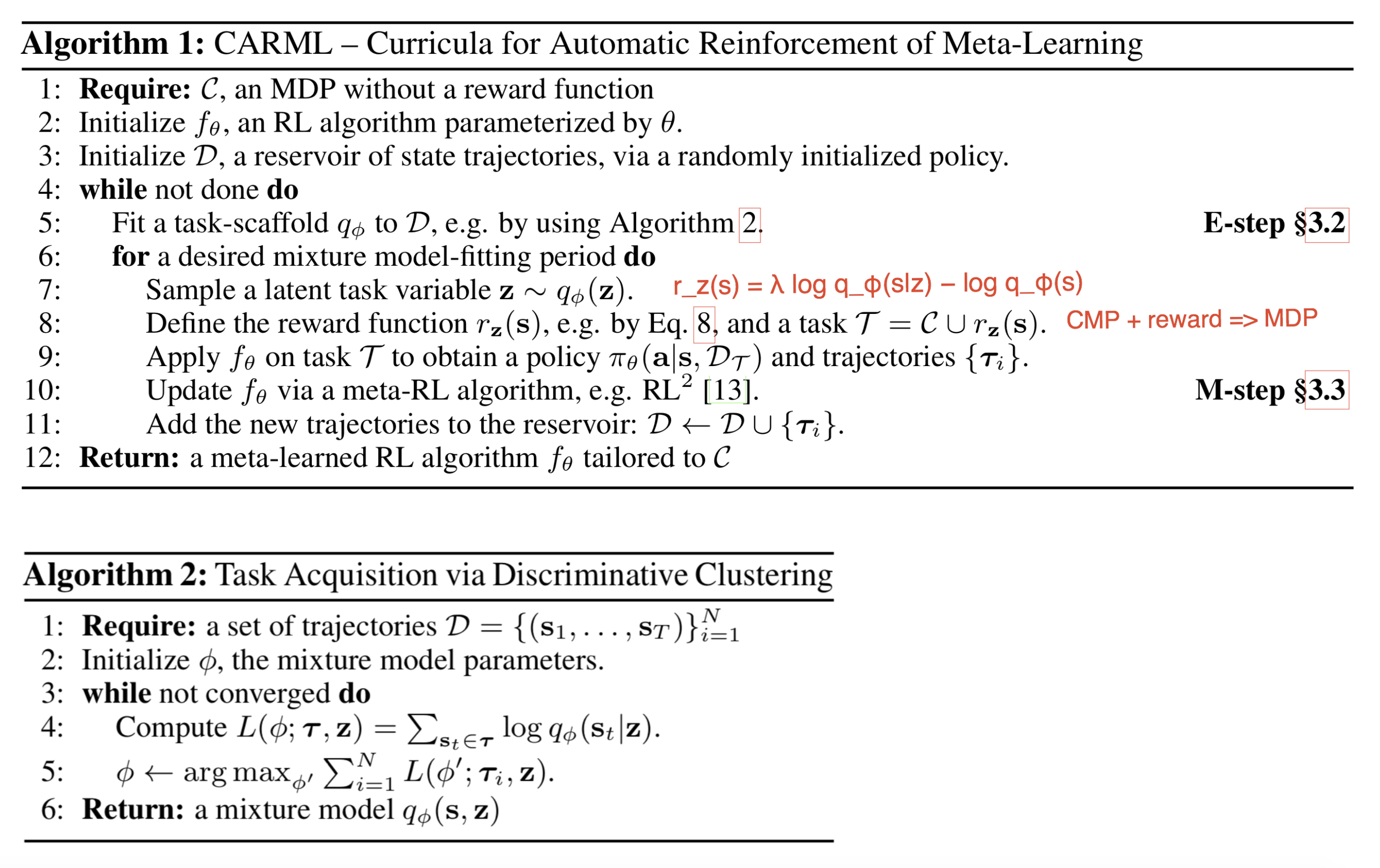 Fig. 9. The algorithm of CARML. (Image source: Jabri, et al 2019)
Learning a latent skill space can be done in different ways, such as in Hausman, et al. 2018. The goal of their approach is to learn a task-conditioned policy, $\pi(a \vert s, t^{(i)})$, where $t^{(i)}$ is from a discrete list of $N$ tasks, $\mathcal{T} = [t^{(1)}, \dots, t^{(N)}]$. However, rather than learning $N$ separate solutions, one per task, it would be nice to learn a latent skill space so that each task could be represented in a distribution over skills and thus skills are reused between tasks. The policy is defined as $\pi_\theta(a \vert s,t) = \int \pi_\theta(a \vert z,s,t) p_\phi(z \vert t)\mathrm{d}z$, where $\pi_\theta$ and $p_\phi$ are policy and embedding networks to learn, respectively. If $z$ is discrete, i.e. drawn from a set of $K$ skills, then the policy becomes a mixture of $K$ sub-policies. The policy training uses SAC and the dependency on $z$ is introduced in the entropy term.
Curriculum through Distillation
The motivation for the progressive neural network (Rusu et al. 2016) architecture is to efficiently transfer learned skills between different tasks and in the meantime avoid catastrophic forgetting. The curriculum is realized through a set of progressively stacked neural network towers (or “columns”, as in the paper).
A progressive network has the following structure:
- It starts with a single column containing $L$ layers of neurons, in which the corresponding activation layers are labelled as $h^{(1)}_i, i=1, \dots, L$. We first train this single-column network for one task to convergence, achieving parameter config $\theta^{(1)}$.
- Once switch to the next task, we need to add a new column to adapt to the new context while freezing $\theta^{(1)}$ to lock down the learned skills from the previous task. The new column has activation layers labelled as $h^{(2)}_i, i=1, \dots, L$, and parameters $\theta^{(2)}$.
- Step 2 can be repeated with every new task. The $i$-th layer activation in the $k$-th column depends on the previous activation layers in all the existing columns:
where $W^{(k)}_i$ is the weight matrix of the layer $i$ in the column $k$; $U_i^{(k:j)}, j < k$ are the weight matrices for projecting the layer $i-1$ of the column $j$ to the layer $i$ of column $k$ ($ j < k $). The above weights matrices should be learned. $f(.)$ is a non-linear activation function by choice.
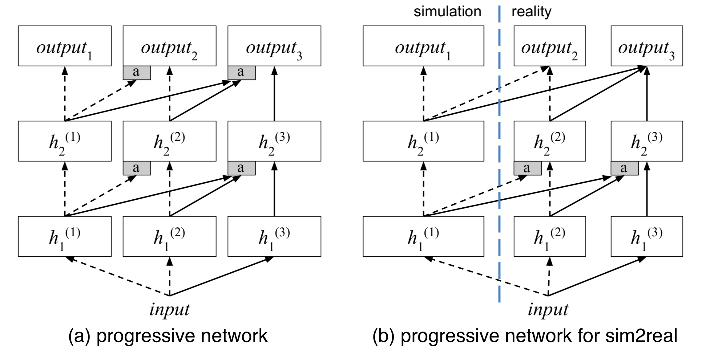 Fig. 10. The progressive neural network architecture. (Image source: Rusu, et al. 2017)
The paper experimented with Atari games by training a progressive network on multiple games to check whether features learned in one game can transfer to another. That is indeed the case. Though interestingly, learning a high dependency on features in the previous columns does not always indicate good transfer performance on the new task. One hypothesis is that features learned from the old task might introduce biases into the new task, leading to policy getting trapped in a sub-optimal solution. Overall, the progressive network works better than only fine-tuning the top layer and can achieve similar transfer performance as fine-tuning the entire network.
One use case for the progressive network is to do sim2real transfer (Rusu, et al. 2017), in which the first column is trained in simulator with a lot of samples and then the additional columns (could be for different real-world tasks) are added and trained with a few real data samples.
Czarnecki, et al. (2018) proposed another RL training framework, Mix and Match (short for M&M) to provide curriculum through coping knowledge between agents. Given a sequence of agents from simple to complex, $\pi_1, \dots, \pi_K$, each parameterized with some shared weights (e.g. by shared some lower common layers). M&M trains a mixture of agents, but only the final performance of the most complex one $\pi_K$ matters.
In the meantime, M&M learns a categorical distribution $c \sim \text{Categorical}(1, \dots, K \vert \alpha)$ with pmf $p(c=i) = \alpha_i$ probability to pick which policy to use at a given time. The mixed M&M policy is a simple weighted sum: $\pi_\text{mm}(a \vert s) = \sum_{i=1}^K \alpha_i \pi_i(a \vert s)$. Curriculum learning is realized by dynamically adjusting $\alpha_i$, from $\alpha_K=0$ to $\alpha_K=1$. The tuning of $\alpha$ can be manual or through population-based training.
To encourage cooperation rather than competition among policies, besides the RL loss $\mathcal{L}_\text{RL}$, another distillation -like loss $\mathcal{L}_\text{mm}(\theta)$ is added. The knowledge transfer loss $\mathcal{L}_\text{mm}(\theta)$ measures the KL divergence between two policies, $\propto D_\text{KL}(\pi_{i}(. \vert s) | \pi_j(. \vert s))$ for $i < j$. It encourages complex agents to match the simpler ones early on. The final loss is $\mathcal{L} = \mathcal{L}_\text{RL}(\theta \vert \pi_\text{mm}) + \lambda \mathcal{L}_\text{mm}(\theta)$.
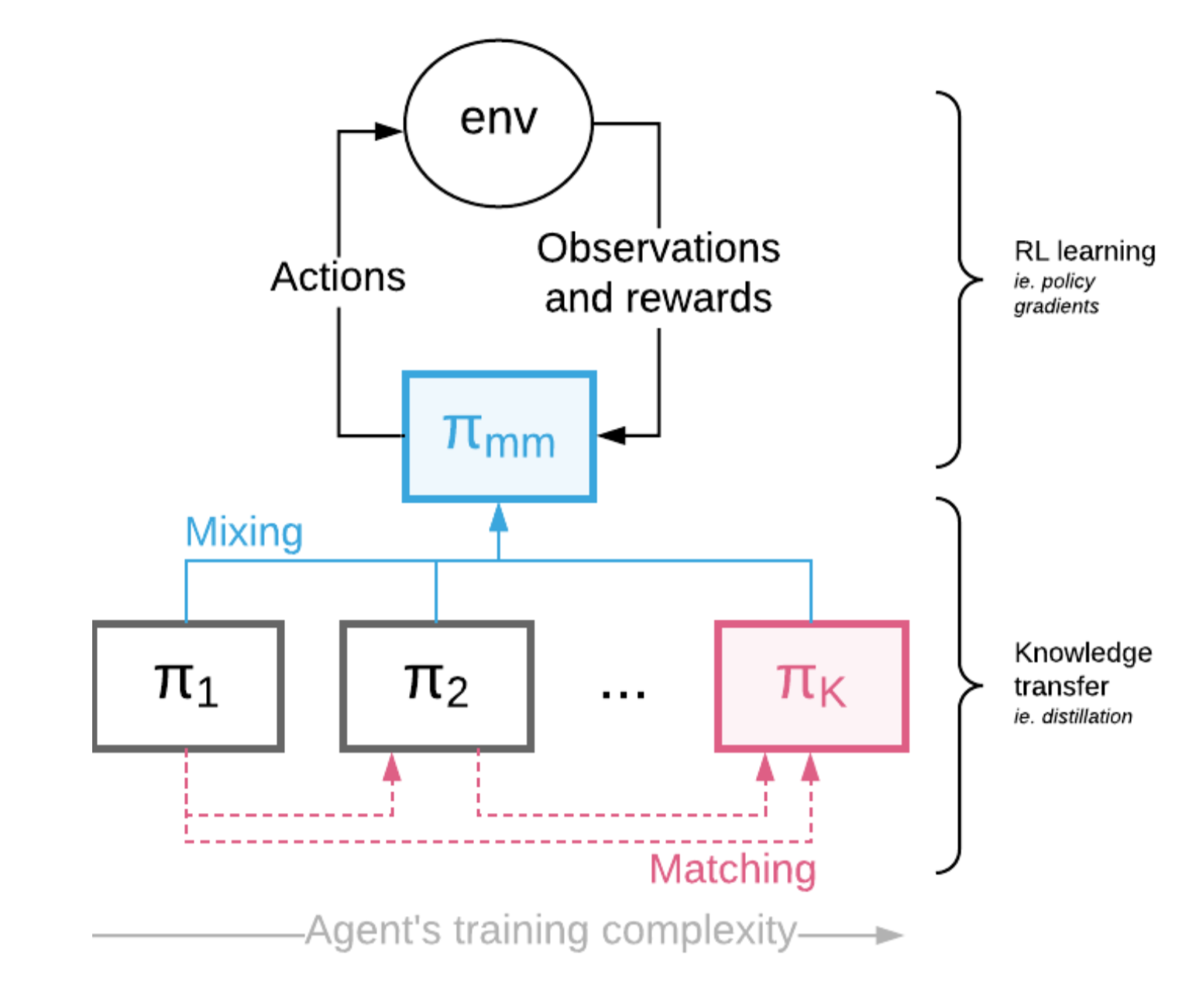 Fig. 11. The Mix & Match architecture for training a mixture of policies. (Image source:Czarnecki, et al., 2018)