Meta Learning

• Define the Meta-Learning Problem
  • A Simple View
  • Training in the Same Way as Testing
  • Learner and Meta-Learner
  • Common Approaches
• Metric-Based
  • Convolutional Siamese Neural Network
  • Matching Networks
    • Simple Embedding
    • Full Context Embeddings
  • Relation Network
  • Prototypical Networks
• Model-Based
  • Memory-Augmented Neural Networks
    • MANN for Meta-Learning
    • Addressing Mechanism for Meta-Learning
  • Meta Networks
    • Fast Weights
    • Model Components
    • Training Process
• Optimization-Based
  • LSTM Meta-Learner
    • Why LSTM?
    • Model Setup
  • MAML
    • First-Order MAML
  • Reptile
    • The Optimization Assumption
    • Reptile vs FOMAML

A good machine learning model often requires training with a large number of samples. Humans, in contrast, learn new concepts and skills much faster and more efficiently. Kids who have seen cats and birds only a few times can quickly tell them apart. People who know how to ride a bike are likely to discover the way to ride a motorcycle fast with little or even no demonstration. Is it possible to design a machine learning model with similar properties - learning new concepts and skills fast with a few training examples? That’s essentially what meta-learning aims to solve.

We expect a good meta-learning model capable of well adapting or generalizing to new tasks and new environments that have never been encountered during training time. The adaptation process, essentially a mini learning session, happens during test but with a limited exposure to the new task configurations. Eventually, the adapted model can complete new tasks. This is why meta-learning is also known as learning to learn.

The tasks can be any well-defined family of machine learning problems: supervised learning, reinforcement learning, etc. For example, here are a couple concrete meta-learning tasks:

• A classifier trained on non-cat images can tell whether a given image contains a cat after seeing a handful of cat pictures.
• A game bot is able to quickly master a new game.
• A mini robot completes the desired task on an uphill surface during test even through it was only trained in a flat surface environment.

Define the Meta-Learning Problem

In this post, we focus on the case when each desired task is a supervised learning problem like image classification. There is a lot of interesting literature on meta-learning with reinforcement learning problems (aka “Meta Reinforcement Learning”), but we would not cover them here.

A Simple View

A good meta-learning model should be trained over a variety of learning tasks and optimized for the best performance on a distribution of tasks, including potentially unseen tasks. Each task is associated with a dataset $\mathcal{D}$, containing both feature vectors and true labels. The optimal model parameters are:

$$\theta^* = \arg\min_\theta \mathbb{E}_{\mathcal{D}\sim p(\mathcal{D})} [\mathcal{L}_\theta(\mathcal{D})]$$

It looks very similar to a normal learning task, but one dataset is considered as one data sample.

Few-shot classification is an instantiation of meta-learning in the field of supervised learning. The dataset $\mathcal{D}$ is often split into two parts, a support set $S$ for learning and a prediction set $B$ for training or testing, $\mathcal{D}=\langle S, B\rangle$. Often we consider a K-shot N-class classification task: the support set contains K labelled examples for each of N classes.

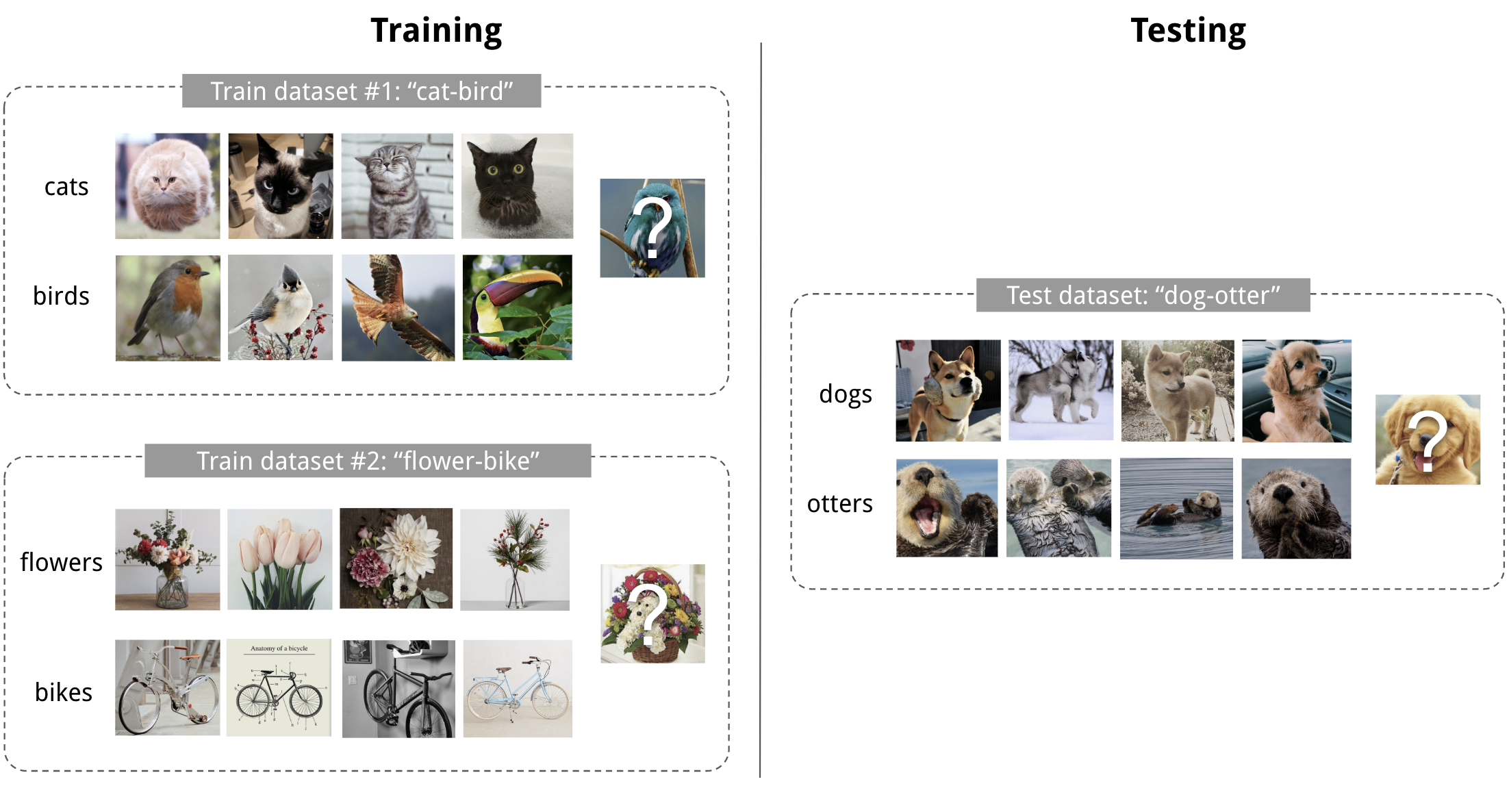
Fig. 1. An example of 4-shot 2-class image classification. (Image thumbnails are from Pinterest)

Training in the Same Way as Testing

A dataset $\mathcal{D}$ contains pairs of feature vectors and labels, $\mathcal{D} = {(\mathbf{x}_i, y_i)}$ and each label belongs to a known label set $\mathcal{L}^\text{label}$. Let’s say, our classifier $f_\theta$ with parameter $\theta$ outputs a probability of a data point belonging to the class $y$ given the feature vector $\mathbf{x}$, $P_\theta(y \vert \mathbf{x})$.

The optimal parameters should maximize the probability of true labels across multiple training batches $B \subset \mathcal{D}$:

$$\begin{aligned} \theta^* &= {\arg\max}_{\theta} \mathbb{E}_{(\mathbf{x}, y)\in \mathcal{D}}[P_\theta(y \vert \mathbf{x})] &\\ \theta^* &= {\arg\max}_{\theta} \mathbb{E}_{B\subset \mathcal{D}}[\sum_{(\mathbf{x}, y)\in B}P_\theta(y \vert \mathbf{x})] & \scriptstyle{\text{; trained with mini-batches.}} \end{aligned}$$

In few-shot classification, the goal is to reduce the prediction error on data samples with unknown labels given a small support set for “fast learning” (think of how “fine-tuning” works). To make the training process mimics what happens during inference, we would like to “fake” datasets with a subset of labels to avoid exposing all the labels to the model and modify the optimization procedure accordingly to encourage fast learning:

1. Sample a subset of labels, $L \subset \mathcal{L}^\text{label}$.
2. Sample a support set $S^L \subset \mathcal{D}$ and a training batch $B^L \subset \mathcal{D}$. Both of them only contain data points with labels belonging to the sampled label set $L$, $y \in L, \forall (x, y) \in S^L, B^L$.
3. The support set is part of the model input.
4. The final optimization uses the mini-batch $B^L$ to compute the loss and update the model parameters through backpropagation, in the same way as how we use it in the supervised learning.

You may consider each pair of sampled dataset $(S^L, B^L)$ as one data point. The model is trained such that it can generalize to other datasets. Symbols in red are added for meta-learning in addition to the supervised learning objective.

$$\theta = \arg\max_\theta \color{red}{E_{L\subset\mathcal{L}}[} E_{\color{red}{S^L \subset\mathcal{D}, }B^L \subset\mathcal{D}} [\sum_{(x, y)\in B^L} P_\theta(x, y\color{red}{, S^L})] \color{red}{]}$$

The idea is to some extent similar to using a pre-trained model in image classification (ImageNet) or language modeling (big text corpora) when only a limited set of task-specific data samples are available. Meta-learning takes this idea one step further, rather than fine-tuning according to one down-steam task, it optimizes the model to be good at many, if not all.

Learner and Meta-Learner

Another popular view of meta-learning decomposes the model update into two stages:

• A classifier $f_\theta$ is the “learner” model, trained for operating a given task;
• In the meantime, a optimizer $g_\phi$ learns how to update the learner model’s parameters via the support set $S$, $\theta’ = g_\phi(\theta, S)$.

Then in final optimization step, we need to update both $\theta$ and $\phi$ to maximize:

$$\mathbb{E}_{L\subset\mathcal{L}}[ \mathbb{E}_{S^L \subset\mathcal{D}, B^L \subset\mathcal{D}} [\sum_{(\mathbf{x}, y)\in B^L} P_{g_\phi(\theta, S^L)}(y \vert \mathbf{x})]]$$

Common Approaches

There are three common approaches to meta-learning: metric-based, model-based, and optimization-based. Oriol Vinyals has a nice summary in his talk at meta-learning symposium @ NIPS 2018:

	Model-based	Metric-based	Optimization-based
Key idea	RNN; memory	Metric learning	Gradient descent
How $P_\theta(y \vert \mathbf{x})$ is modeled?	$f_\theta(\mathbf{x}, S)$	$\sum_{(\mathbf{x}_i, y_i) \in S} k_\theta(\mathbf{x}, \mathbf{x}_i)y_i$ (*)	$P_{g_\phi(\theta, S^L)}(y \vert \mathbf{x})$

(*) $k_\theta$ is a kernel function measuring the similarity between $\mathbf{x}_i$ and $\mathbf{x}$.

Next we are gonna review classic models in each approach.

Metric-Based

The core idea in metric-based meta-learning is similar to nearest neighbors algorithms (i.e., k-NN classificer and k-means clustering) and kernel density estimation. The predicted probability over a set of known labels $y$ is a weighted sum of labels of support set samples. The weight is generated by a kernel function $k_\theta$, measuring the similarity between two data samples.

$ P_\theta(y \vert \mathbf{x}, S) = \sum_{(\mathbf{x}_i, y_i) \in S} k_\theta(\mathbf{x}, \mathbf{x}_i)y_i $

To learn a good kernel is crucial to the success of a metric-based meta-learning model. Metric learning is well aligned with this intention, as it aims to learn a metric or distance function over objects. The notion of a good metric is problem-dependent. It should represent the relationship between inputs in the task space and facilitate problem solving.

All the models introduced below learn embedding vectors of input data explicitly and use them to design proper kernel functions.

Convolutional Siamese Neural Network

The Siamese Neural Network is composed of two twin networks and their outputs are jointly trained on top with a function to learn the relationship between pairs of input data samples. The twin networks are identical, sharing the same weights and network parameters. In other words, both refer to the same embedding network that learns an efficient embedding to reveal relationship between pairs of data points.

Koch, Zemel & Salakhutdinov (2015) proposed a method to use the siamese neural network to do one-shot image classification. First, the siamese network is trained for a verification task for telling whether two input images are in the same class. It outputs the probability of two images belonging to the same class. Then, during test time, the siamese network processes all the image pairs between a test image and every image in the support set. The final prediction is the class of the support image with the highest probability.

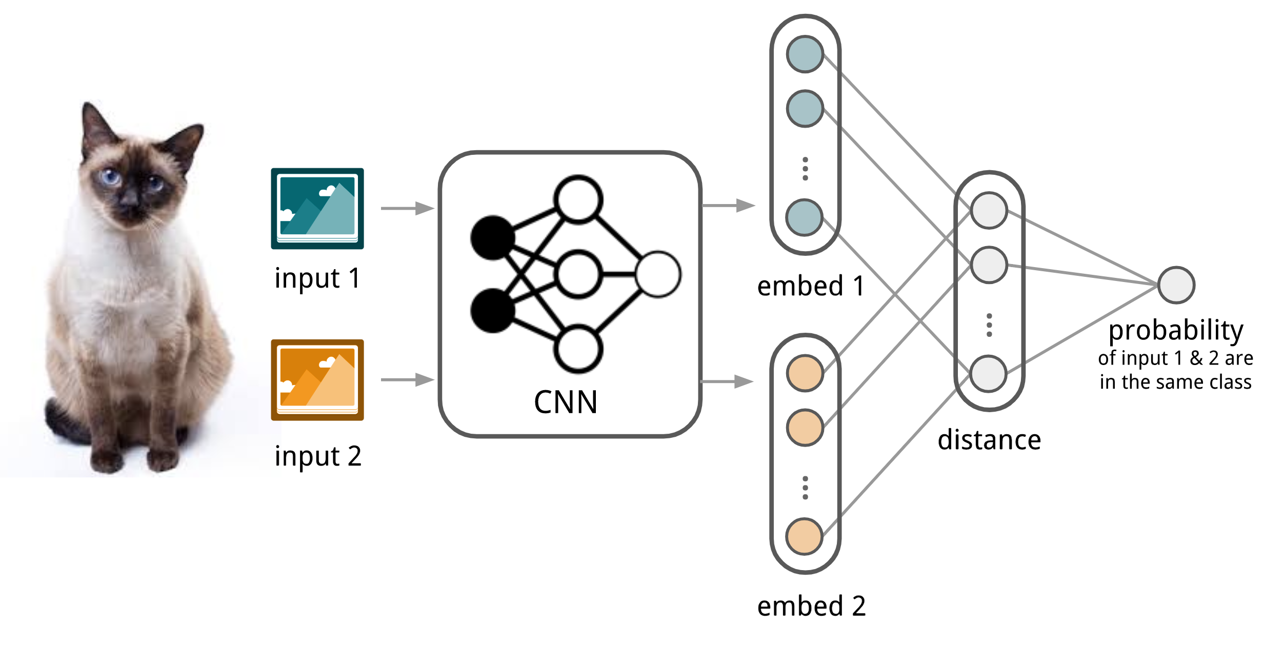
Fig. 2. The architecture of convolutional siamese neural network for few-show image classification.

1. First, convolutional siamese network learns to encode two images into feature vectors via a embedding function $f_\theta$ which contains a couple of convolutional layers.
2. The L1-distance between two embeddings is $\vert f_\theta(\mathbf{x}_i) - f_\theta(\mathbf{x}_j) \vert$.
3. The distance is converted to a probability $p$ by a linear feedforward layer and sigmoid. It is the probability of whether two images are drawn from the same class.
4. Intuitively the loss is cross entropy because the label is binary.

$$\begin{aligned} p(\mathbf{x}_i, \mathbf{x}_j) &= \sigma(\mathbf{W}\vert f_\theta(\mathbf{x}_i) - f_\theta(\mathbf{x}_j) \vert) \\ \mathcal{L}(B) &= \sum_{(\mathbf{x}_i, \mathbf{x}_j, y_i, y_j)\in B} \mathbf{1}_{y_i=y_j}\log p(\mathbf{x}_i, \mathbf{x}_j) + (1-\mathbf{1}_{y_i=y_j})\log (1-p(\mathbf{x}_i, \mathbf{x}_j)) \end{aligned}$$

Images in the training batch $B$ can be augmented with distortion. Of course, you can replace the L1 distance with other distance metric, L2, cosine, etc. Just make sure they are differential and then everything else works the same.

Given a support set $S$ and a test image $\mathbf{x}$, the final predicted class is:

$$\hat{c}_S(\mathbf{x}) = c(\arg\max_{\mathbf{x}_i \in S} P(\mathbf{x}, \mathbf{x}_i))$$

where $c(\mathbf{x})$ is the class label of an image $\mathbf{x}$ and $\hat{c}(.)$ is the predicted label.

The assumption is that the learned embedding can be generalized to be useful for measuring the distance between images of unknown categories. This is the same assumption behind transfer learning via the adoption of a pre-trained model; for example, the convolutional features learned in the model pre-trained with ImageNet are expected to help other image tasks. However, the benefit of a pre-trained model decreases when the new task diverges from the original task that the model was trained on.

Matching Networks

The task of Matching Networks (Vinyals et al., 2016) is to learn a classifier $c_S$ for any given (small) support set $S={x_i, y_i}_{i=1}^k$ (k-shot classification). This classifier defines a probability distribution over output labels $y$ given a test example $\mathbf{x}$. Similar to other metric-based models, the classifier output is defined as a sum of labels of support samples weighted by attention kernel $a(\mathbf{x}, \mathbf{x}_i)$ - which should be proportional to the similarity between $\mathbf{x}$ and $\mathbf{x}_i$.

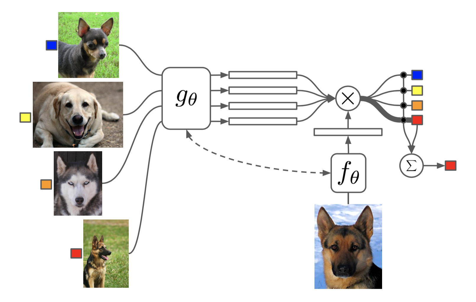
Fig. 3. The architecture of Matching Networks. (Image source: original paper)

$$c_S(\mathbf{x}) = P(y \vert \mathbf{x}, S) = \sum_{i=1}^k a(\mathbf{x}, \mathbf{x}_i) y_i \text{, where }S=\{(\mathbf{x}_i, y_i)\}_{i=1}^k$$

The attention kernel depends on two embedding functions, $f$ and $g$, for encoding the test sample and the support set samples respectively. The attention weight between two data points is the cosine similarity, $\text{cosine}(.)$, between their embedding vectors, normalized by softmax:

$$a(\mathbf{x}, \mathbf{x}_i) = \frac{\exp(\text{cosine}(f(\mathbf{x}), g(\mathbf{x}_i))}{\sum_{j=1}^k\exp(\text{cosine}(f(\mathbf{x}), g(\mathbf{x}_j))}$$

Simple Embedding

In the simple version, an embedding function is a neural network with a single data sample as input. Potentially we can set $f=g$.

Full Context Embeddings

The embedding vectors are critical inputs for building a good classifier. Taking a single data point as input might not be enough to efficiently gauge the entire feature space. Therefore, the Matching Network model further proposed to enhance the embedding functions by taking as input the whole support set $S$ in addition to the original input, so that the learned embedding can be adjusted based on the relationship with other support samples.

• $g_\theta(\mathbf{x}_i, S)$ uses a bidirectional LSTM to encode $\mathbf{x}_i$ in the context of the entire support set $S$.

• $f_\theta(\mathbf{x}, S)$ encodes the test sample $\mathbf{x}$ visa an LSTM with read attention over the support set $S$.

  1. First the test sample goes through a simple neural network, such as a CNN, to extract basic features, $f’(\mathbf{x})$.
  2. Then an LSTM is trained with a read attention vector over the support set as part of the hidden state:
  $$\begin{aligned} \hat{\mathbf{h}}_t, \mathbf{c}_t &= \text{LSTM}(f'(\mathbf{x}), [\mathbf{h}_{t-1}, \mathbf{r}_{t-1}], \mathbf{c}_{t-1}) \\ \mathbf{h}_t &= \hat{\mathbf{h}}_t + f'(\mathbf{x}) \\ \mathbf{r}_{t-1} &= \sum_{i=1}^k a(\mathbf{h}_{t-1}, g(\mathbf{x}_i)) g(\mathbf{x}_i) \\ a(\mathbf{h}_{t-1}, g(\mathbf{x}_i)) &= \text{softmax}(\mathbf{h}_{t-1}^\top g(\mathbf{x}_i)) = \frac{\exp(\mathbf{h}_{t-1}^\top g(\mathbf{x}_i))}{\sum_{j=1}^k \exp(\mathbf{h}_{t-1}^\top g(\mathbf{x}_j))} \end{aligned}$$
  1. Eventually $f(\mathbf{x}, S)=\mathbf{h}_K$ if we do K steps of “read”.

This embedding method is called “Full Contextual Embeddings (FCE)”. Interestingly it does help improve the performance on a hard task (few-shot classification on mini ImageNet), but makes no difference on a simple task (Omniglot).

The training process in Matching Networks is designed to match inference at test time, see the details in the earlier section. It is worthy of mentioning that the Matching Networks paper refined the idea that training and testing conditions should match.

$$\theta^* = \arg\max_\theta \mathbb{E}_{L\subset\mathcal{L}}[ \mathbb{E}_{S^L \subset\mathcal{D}, B^L \subset\mathcal{D}} [\sum_{(\mathbf{x}, y)\in B^L} P_\theta(y\vert\mathbf{x}, S^L)]]$$

Relation Network

Relation Network (RN) (Sung et al., 2018) is similar to siamese network but with a few differences:

1. The relationship is not captured by a simple L1 distance in the feature space, but predicted by a CNN classifier $g_\phi$. The relation score between a pair of inputs, $\mathbf{x}_i$ and $\mathbf{x}_j$, is $r_{ij} = g_\phi([\mathbf{x}_i, \mathbf{x}_j])$ where $[.,.]$ is concatenation.
2. The objective function is MSE loss instead of cross-entropy, because conceptually RN focuses more on predicting relation scores which is more like regression, rather than binary classification, $\mathcal{L}(B) = \sum_{(\mathbf{x}_i, \mathbf{x}_j, y_i, y_j)\in B} (r_{ij} - \mathbf{1}_{y_i=y_j})^2$.

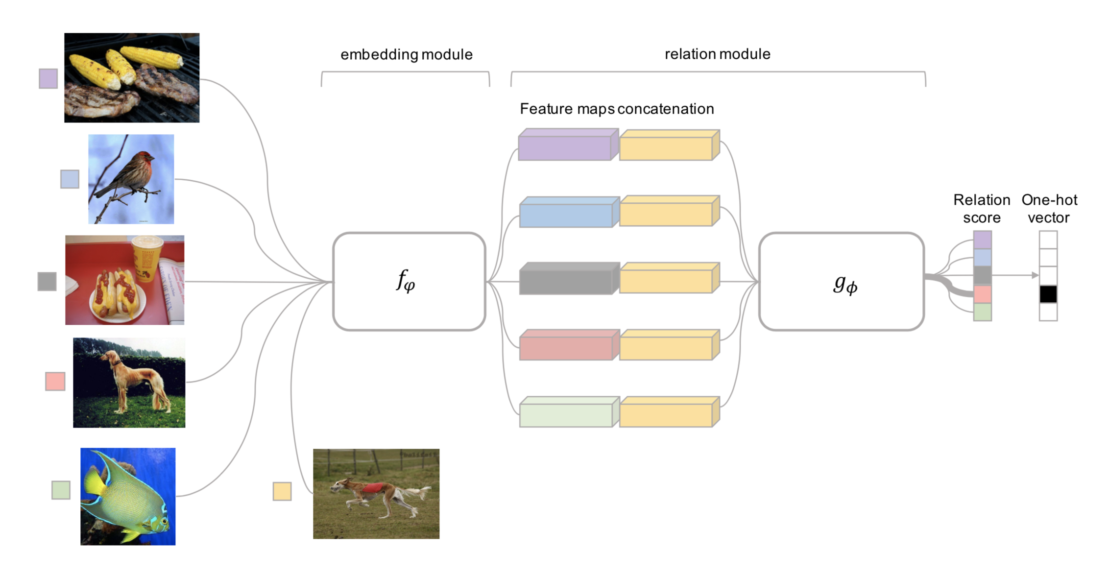
Fig. 4. Relation Network architecture for a 5-way 1-shot problem with one query example. (Image source: original paper)

(Note: There is another Relation Network for relational reasoning, proposed by DeepMind. Don’t get confused.)

Prototypical Networks

Prototypical Networks (Snell, Swersky & Zemel, 2017) use an embedding function $f_\theta$ to encode each input into a $M$-dimensional feature vector. A prototype feature vector is defined for every class $c \in \mathcal{C}$, as the mean vector of the embedded support data samples in this class.

$$\mathbf{v}_c = \frac{1}{|S_c|} \sum_{(\mathbf{x}_i, y_i) \in S_c} f_\theta(\mathbf{x}_i)$$

Fig. 5. Prototypical networks in the few-shot and zero-shot scenarios. (Image source: original paper)

The distribution over classes for a given test input $\mathbf{x}$ is a softmax over the inverse of distances between the test data embedding and prototype vectors.

$$P(y=c\vert\mathbf{x})=\text{softmax}(-d_\varphi(f_\theta(\mathbf{x}), \mathbf{v}_c)) = \frac{\exp(-d_\varphi(f_\theta(\mathbf{x}), \mathbf{v}_c))}{\sum_{c' \in \mathcal{C}}\exp(-d_\varphi(f_\theta(\mathbf{x}), \mathbf{v}_{c'}))}$$

where $d_\varphi$ can be any distance function as long as $\varphi$ is differentiable. In the paper, they used the squared euclidean distance.

The loss function is the negative log-likelihood: $\mathcal{L}(\theta) = -\log P_\theta(y=c\vert\mathbf{x})$.

Model-Based

Model-based meta-learning models make no assumption on the form of $P_\theta(y\vert\mathbf{x})$. Rather it depends on a model designed specifically for fast learning — a model that updates its parameters rapidly with a few training steps. This rapid parameter update can be achieved by its internal architecture or controlled by another meta-learner model.

Memory-Augmented Neural Networks

A family of model architectures use external memory storage to facilitate the learning process of neural networks, including Neural Turing Machines and Memory Networks. With an explicit storage buffer, it is easier for the network to rapidly incorporate new information and not to forget in the future. Such a model is known as MANN, short for “Memory-Augmented Neural Network”. Note that recurrent neural networks with only internal memory such as vanilla RNN or LSTM are not MANNs.

Because MANN is expected to encode new information fast and thus to adapt to new tasks after only a few samples, it fits well for meta-learning. Taking the Neural Turing Machine (NTM) as the base model, Santoro et al. (2016) proposed a set of modifications on the training setup and the memory retrieval mechanisms (or “addressing mechanisms”, deciding how to assign attention weights to memory vectors). Please go through the NTM section in my other post first if you are not familiar with this matter before reading forward.

As a quick recap, NTM couples a controller neural network with external memory storage. The controller learns to read and write memory rows by soft attention, while the memory serves as a knowledge repository. The attention weights are generated by its addressing mechanism: content-based + location based.

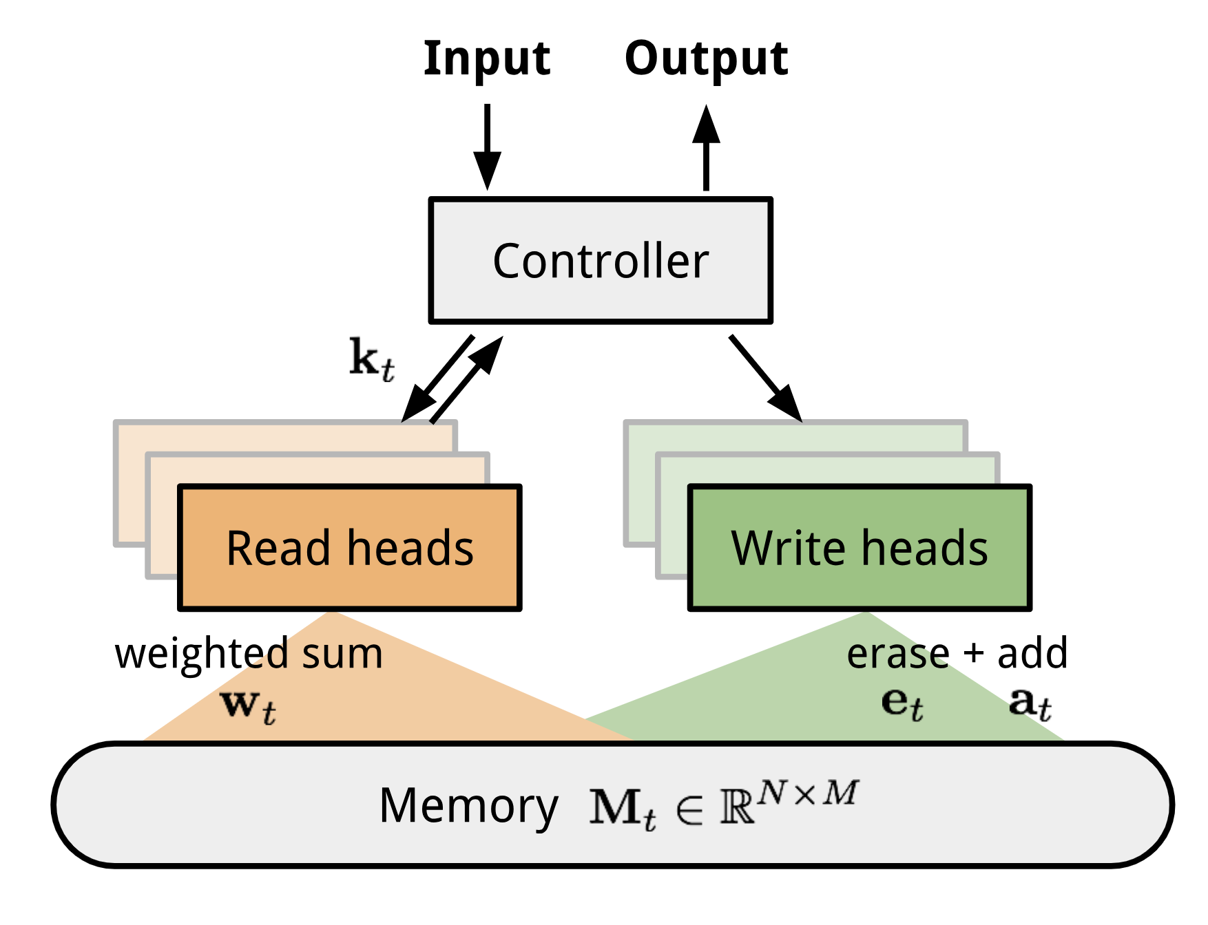
Fig. 6. The architecture of Neural Turing Machine (NTM). The memory at time t, $\mathbf{M}_t$ is a matrix of size $N \times M$, containing N vector rows and each has M dimensions.

MANN for Meta-Learning

To use MANN for meta-learning tasks, we need to train it in a way that the memory can encode and capture information of new tasks fast and, in the meantime, any stored representation is easily and stably accessible.

The training described in Santoro et al., 2016 happens in an interesting way so that the memory is forced to hold information for longer until the appropriate labels are presented later. In each training episode, the truth label $y_t$ is presented with one step offset, $(\mathbf{x}_{t+1}, y_t)$: it is the true label for the input at the previous time step t, but presented as part of the input at time step t+1.

Fig. 7. Task setup in MANN for meta-learning (Image source: original paper).

In this way, MANN is motivated to memorize the information of a new dataset, because the memory has to hold the current input until the label is present later and then retrieve the old information to make a prediction accordingly.

Next let us see how the memory is updated for efficient information retrieval and storage.

Addressing Mechanism for Meta-Learning

Aside from the training process, a new pure content-based addressing mechanism is utilized to make the model better suitable for meta-learning.

How to read from memory?
The read attention is constructed purely based on the content similarity.

First, a key feature vector $\mathbf{k}_t$ is produced at the time step t by the controller as a function of the input $\mathbf{x}$. Similar to NTM, a read weighting vector $\mathbf{w}_t^r$ of N elements is computed as the cosine similarity between the key vector and every memory vector row, normalized by softmax. The read vector $\mathbf{r}_t$ is a sum of memory records weighted by such weightings:

$$\mathbf{r}_i = \sum_{i=1}^N w_t^r(i)\mathbf{M}_t(i) \text{, where } w_t^r(i) = \text{softmax}(\frac{\mathbf{k}_t \cdot \mathbf{M}_t(i)}{\|\mathbf{k}_t\| \cdot \|\mathbf{M}_t(i)\|})$$

where $M_t$ is the memory matrix at time t and $M_t(i)$ is the i-th row in this matrix.

How to write into memory?
The addressing mechanism for writing newly received information into memory operates a lot like the cache replacement policy. The Least Recently Used Access (LRUA) writer is designed for MANN to better work in the scenario of meta-learning. A LRUA write head prefers to write new content to either the least used memory location or the most recently used memory location.

• Rarely used locations: so that we can preserve frequently used information (see LFU);
• The last used location: the motivation is that once a piece of information is retrieved once, it probably won’t be called again for a while (see MRU).

There are many cache replacement algorithms and each of them could potentially replace the design here with better performance in different use cases. Furthermore, it would be a good idea to learn the memory usage pattern and addressing strategies rather than arbitrarily set it.

The preference of LRUA is carried out in a way that everything is differentiable:

1. The usage weight $\mathbf{w}^u_t$ at time t is a sum of current read and write vectors, in addition to the decayed last usage weight, $\gamma \mathbf{w}^u_{t-1}$, where $\gamma$ is a decay factor.
2. The write vector is an interpolation between the previous read weight (prefer “the last used location”) and the previous least-used weight (prefer “rarely used location”). The interpolation parameter is the sigmoid of a hyperparameter $\alpha$.
3. The least-used weight $\mathbf{w}^{lu}$ is scaled according to usage weights $\mathbf{w}_t^u$, in which any dimension remains at 1 if smaller than the n-th smallest element in the vector and 0 otherwise.

$$\begin{aligned} \mathbf{w}_t^u &= \gamma \mathbf{w}_{t-1}^u + \mathbf{w}_t^r + \mathbf{w}_t^w \\ \mathbf{w}_t^r &= \text{softmax}(\text{cosine}(\mathbf{k}_t, \mathbf{M}_t(i))) \\ \mathbf{w}_t^w &= \sigma(\alpha)\mathbf{w}_{t-1}^r + (1-\sigma(\alpha))\mathbf{w}^{lu}_{t-1}\\ \mathbf{w}_t^{lu} &= \mathbf{1}_{w_t^u(i) \leq m(\mathbf{w}_t^u, n)} \text{, where }m(\mathbf{w}_t^u, n)\text{ is the }n\text{-th smallest element in vector }\mathbf{w}_t^u\text{.} \end{aligned}$$

Finally, after the least used memory location, indicated by $\mathbf{w}_t^{lu}$, is set to zero, every memory row is updated:

$$\mathbf{M}_t(i) = \mathbf{M}_{t-1}(i) + w_t^w(i)\mathbf{k}_t, \forall i$$

Meta Networks

Meta Networks (Munkhdalai & Yu, 2017), short for MetaNet, is a meta-learning model with architecture and training process designed for rapid generalization across tasks.

Fast Weights

The rapid generalization of MetaNet relies on “fast weights”. There are a handful of papers on this topic, but I haven’t read all of them in detail and I failed to find a very concrete definition, only a vague agreement on the concept. Normally weights in the neural networks are updated by stochastic gradient descent in an objective function and this process is known to be slow. One faster way to learn is to utilize one neural network to predict the parameters of another neural network and the generated weights are called fast weights. In comparison, the ordinary SGD-based weights are named slow weights.

In MetaNet, loss gradients are used as meta information to populate models that learn fast weights. Slow and fast weights are combined to make predictions in neural networks.

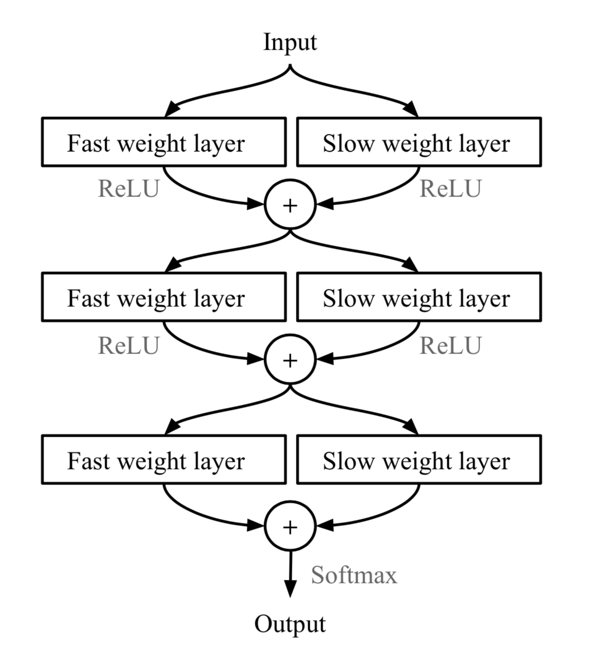
Fig. 8. Combining slow and fast weights in a MLP. $\bigoplus$ is element-wise sum. (Image source: original paper).

Model Components

Disclaimer: Below you will find my annotations are different from those in the paper. imo, the paper is poorly written, but the idea is still interesting. So I’m presenting the idea in my own language.

Key components of MetaNet are:

• An embedding function $f_\theta$, parameterized by $\theta$, encodes raw inputs into feature vectors. Similar to Siamese Neural Network, these embeddings are trained to be useful for telling whether two inputs are of the same class (verification task).
• A base learner model $g_\phi$, parameterized by weights $\phi$, completes the actual learning task.

If we stop here, it looks just like Relation Network. MetaNet, in addition, explicitly models the fast weights of both functions and then aggregates them back into the model (See Fig. 8).

Therefore we need additional two functions to output fast weights for $f$ and $g$ respectively.

• $F_w$: a LSTM parameterized by $w$ for learning fast weights $\theta^+$ of the embedding function $f$. It takes as input gradients of $f$’s embedding loss for verification task.
• $G_v$: a neural network parameterized by $v$ learning fast weights $\phi^+$ for the base learner $g$ from its loss gradients. In MetaNet, the learner’s loss gradients are viewed as the meta information of the task.

Ok, now let’s see how meta networks are trained. The training data contains multiple pairs of datasets: a support set $S=\{\mathbf{x}’_i, y’_i\}_{i=1}^K$ and a test set $U=\{\mathbf{x}_i, y_i\}_{i=1}^L$. Recall that we have four networks and four sets of model parameters to learn, $(\theta, \phi, w, v)$.

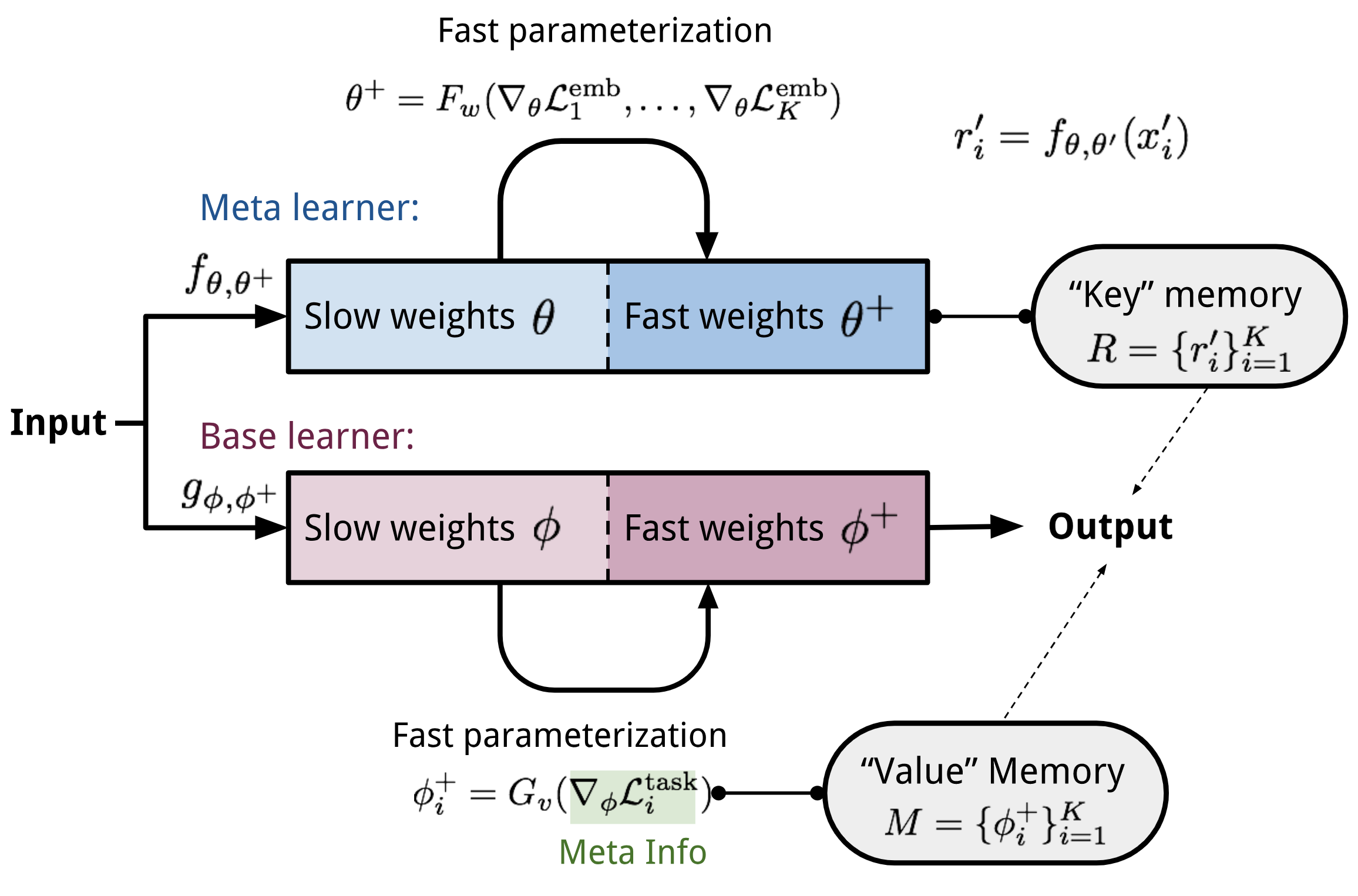
Fig.9. The MetaNet architecture.

Training Process

1. Sample a random pair of inputs at each time step t from the support set $S$, $(\mathbf{x}’_i, y’_i)$ and $(\mathbf{x}’_j, y_j)$. Let $\mathbf{x}_{(t,1)}=\mathbf{x}’_i$ and $\mathbf{x}_{(t,2)}=\mathbf{x}’_j$.
   for $t = 1, \dots, K$:

   a. Compute a loss for representation learning; i.e., cross entropy for the verification task:
   $\mathcal{L}^\text{emb}_t = \mathbf{1}_{y’_i=y’_j} \log P_t + (1 - \mathbf{1}_{y’_i=y’_j})\log(1 - P_t)\text{, where }P_t = \sigma(\mathbf{W}\vert f_\theta(\mathbf{x}_{(t,1)}) - f_\theta(\mathbf{x}_{(t,2)})\vert)$

2. Compute the task-level fast weights: $\theta^+ = F_w(\nabla_\theta \mathcal{L}^\text{emb}_1, \dots, \mathcal{L}^\text{emb}_T)$

3. Next go through examples in the support set $S$ and compute the example-level fast weights. Meanwhile, update the memory with learned representations.
   for $i=1, \dots, K$:

   a. The base learner outputs a probability distribution: $P(\hat{y}_i \vert \mathbf{x}_i) = g_\phi(\mathbf{x}_i)$ and the loss can be cross-entropy or MSE: $\mathcal{L}^\text{task}_i = y’_i \log g_\phi(\mathbf{x}’_i) + (1- y’_i) \log (1 - g_\phi(\mathbf{x}’_i))$

   b. Extract meta information (loss gradients) of the task and compute the example-level fast weights: $\phi_i^+ = G_v(\nabla_\phi\mathcal{L}^\text{task}_i)$

   c. Then store $\phi^+_i$ into $i$-th location of the “value” memory $\mathbf{M}$.

   d. Encode the support sample into a task-specific input representation using both slow and fast weights: $r’_i = f_{\theta, \theta^+}(\mathbf{x}’_i)$ Then store $r’_i$ into $i$-th location of the “key” memory $\mathbf{R}$.

4. Finally it is the time to construct the training loss using the test set $U=\{\mathbf{x}_i, y_i\}_{i=1}^L$.
   Starts with $\mathcal{L}_\text{train}=0$:
   for $j=1, \dots, L$:

   a. Encode the test sample into a task-specific input representation: $r_j = f_{\theta, \theta^+}(\mathbf{x}_j)$

   b. The fast weights are computed by attending to representations of support set samples in memory $\mathbf{R}$. The attention function is of your choice. Here MetaNet uses cosine similarity:
   $\begin{aligned} a_j &= \text{cosine}(\mathbf{R}, r_j) = [\frac{r'_1\cdot r_j}{\|r'_1\|\cdot\|r_j\|}, \dots, \frac{r'_N\cdot r_j}{\|r'_N\|\cdot\|r_j\|}]\\ \phi^+_j &= \text{softmax}(a_j)^\top \mathbf{M} \end{aligned}$

   c. Update the training loss: $\mathcal{L}_\text{train} \leftarrow \mathcal{L}_\text{train} + \mathcal{L}^\text{task}(g_{\phi, \phi^+}(\mathbf{x}_i), y_i) $

5. Update all the parameters $(\theta, \phi, w, v)$ using $\mathcal{L}_\text{train}$.

Optimization-Based

Deep learning models learn through backpropagation of gradients. However, the gradient-based optimization is neither designed to cope with a small number of training samples, nor to converge within a small number of optimization steps. Is there a way to adjust the optimization algorithm so that the model can be good at learning with a few examples? This is what optimization-based approach meta-learning algorithms intend for.

LSTM Meta-Learner

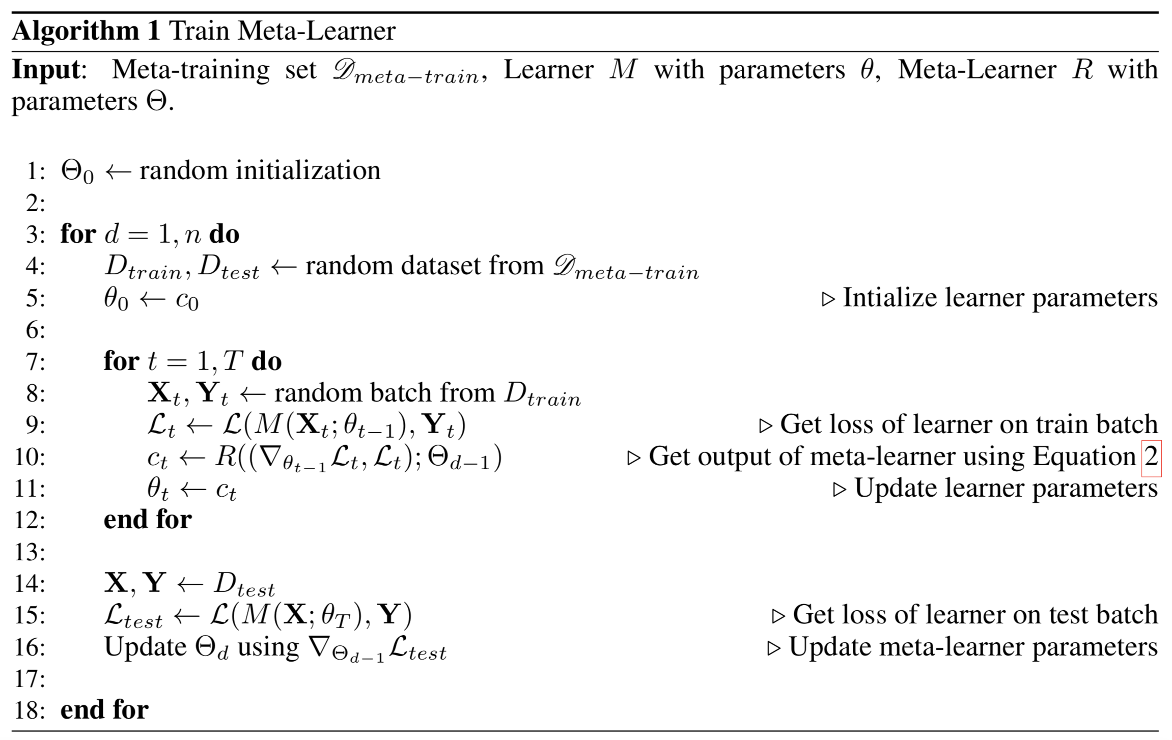
The optimization algorithm can be explicitly modeled. Ravi & Larochelle (2017) did so and named it “meta-learner”, while the original model for handling the task is called “learner”. The goal of the meta-learner is to efficiently update the learner’s parameters using a small support set so that the learner can adapt to the new task quickly.

Let’s denote the learner model as $M_\theta$ parameterized by $\theta$, the meta-learner as $R_\Theta$ with parameters $\Theta$, and the loss function $\mathcal{L}$.

Why LSTM?

The meta-learner is modeled as a LSTM, because:

1. There is similarity between the gradient-based update in backpropagation and the cell-state update in LSTM.
2. Knowing a history of gradients benefits the gradient update; think about how momentum works.

The update for the learner’s parameters at time step t with a learning rate $\alpha_t$ is:

$$\theta_t = \theta_{t-1} - \alpha_t \nabla_{\theta_{t-1}}\mathcal{L}_t$$

It has the same form as the cell state update in LSTM, if we set forget gate $f_t=1$, input gate $i_t = \alpha_t$, cell state $c_t = \theta_t$, and new cell state $\tilde{c}_t = -\nabla_{\theta_{t-1}}\mathcal{L}_t$:

$$\begin{aligned} c_t &= f_t \odot c_{t-1} + i_t \odot \tilde{c}_t\\ &= \theta_{t-1} - \alpha_t\nabla_{\theta_{t-1}}\mathcal{L}_t \end{aligned}$$

While fixing $f_t=1$ and $i_t=\alpha_t$ might not be the optimal, both of them can be learnable and adaptable to different datasets.

$$\begin{aligned} f_t &= \sigma(\mathbf{W}_f \cdot [\nabla_{\theta_{t-1}}\mathcal{L}_t, \mathcal{L}_t, \theta_{t-1}, f_{t-1}] + \mathbf{b}_f) & \scriptstyle{\text{; how much to forget the old value of parameters.}}\\ i_t &= \sigma(\mathbf{W}_i \cdot [\nabla_{\theta_{t-1}}\mathcal{L}_t, \mathcal{L}_t, \theta_{t-1}, i_{t-1}] + \mathbf{b}_i) & \scriptstyle{\text{; corresponding to the learning rate at time step t.}}\\ \tilde{\theta}_t &= -\nabla_{\theta_{t-1}}\mathcal{L}_t &\\ \theta_t &= f_t \odot \theta_{t-1} + i_t \odot \tilde{\theta}_t &\\ \end{aligned}$$

Model Setup

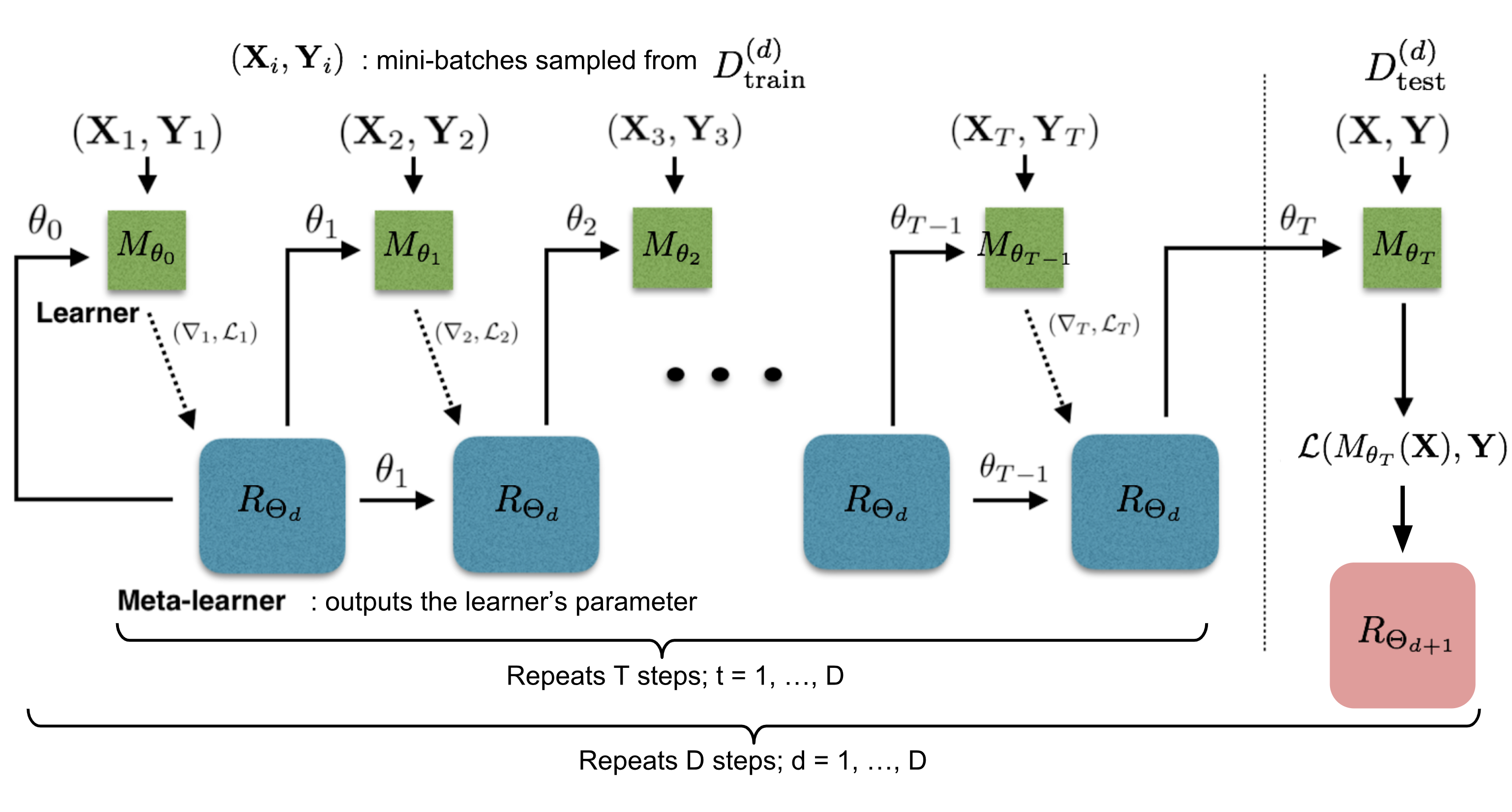
Fig. 10. How the learner $M\_\theta$ and the meta-learner $R\_\Theta$ are trained. (Image source: original paper) with more annotations)

The training process mimics what happens during test, since it has been proved to be beneficial in Matching Networks. During each training epoch, we first sample a dataset $\mathcal{D} = (\mathcal{D}_\text{train}, \mathcal{D}_\text{test}) \in \hat{\mathcal{D}}_\text{meta-train}$ and then sample mini-batches out of $\mathcal{D}_\text{train}$ to update $\theta$ for $T$ rounds. The final state of the learner parameter $\theta_T$ is used to train the meta-learner on the test data $\mathcal{D}_\text{test}$.

Two implementation details to pay extra attention to:

1. How to compress the parameter space in LSTM meta-learner? As the meta-learner is modeling parameters of another neural network, it would have hundreds of thousands of variables to learn. Following the idea of sharing parameters across coordinates,
2. To simplify the training process, the meta-learner assumes that the loss $\mathcal{L}_t$ and the gradient $\nabla_{\theta_{t-1}} \mathcal{L}_t$ are independent.

MAML

MAML, short for Model-Agnostic Meta-Learning (Finn, et al. 2017) is a fairly general optimization algorithm, compatible with any model that learns through gradient descent.

Let’s say our model is $f_\theta$ with parameters $\theta$. Given a task $\tau_i$ and its associated dataset $(\mathcal{D}^{(i)}_\text{train}, \mathcal{D}^{(i)}_\text{test})$, we can update the model parameters by one or more gradient descent steps (the following example only contains one step):

$$\theta'_i = \theta - \alpha \nabla_\theta\mathcal{L}^{(0)}_{\tau_i}(f_\theta)$$

where $\mathcal{L}^{(0)}$ is the loss computed using the mini data batch with id (0).

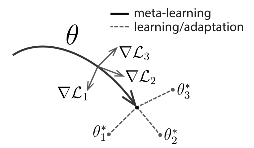
Fig. 11. Diagram of MAML. (Image source: original paper)

Well, the above formula only optimizes for one task. To achieve a good generalization across a variety of tasks, we would like to find the optimal $\theta^*$ so that the task-specific fine-tuning is more efficient. Now, we sample a new data batch with id (1) for updating the meta-objective. The loss, denoted as $\mathcal{L}^{(1)}$, depends on the mini batch (1). The superscripts in $\mathcal{L}^{(0)}$ and $\mathcal{L}^{(1)}$ only indicate different data batches, and they refer to the same loss objective for the same task.

$$\begin{aligned} \theta^* &= \arg\min_\theta \sum_{\tau_i \sim p(\tau)} \mathcal{L}_{\tau_i}^{(1)} (f_{\theta'_i}) = \arg\min_\theta \sum_{\tau_i \sim p(\tau)} \mathcal{L}_{\tau_i}^{(1)} (f_{\theta - \alpha\nabla_\theta \mathcal{L}_{\tau_i}^{(0)}(f_\theta)}) & \\ \theta &\leftarrow \theta - \beta \nabla_{\theta} \sum_{\tau_i \sim p(\tau)} \mathcal{L}_{\tau_i}^{(1)} (f_{\theta - \alpha\nabla_\theta \mathcal{L}_{\tau_i}^{(0)}(f_\theta)}) & \scriptstyle{\text{; updating rule}} \end{aligned}$$

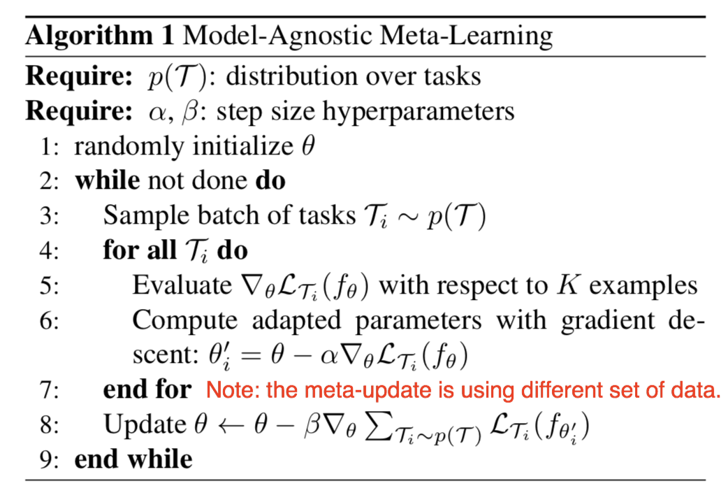
Fig. 12. The general form of MAML algorithm. (Image source: original paper)

First-Order MAML

The meta-optimization step above relies on second derivatives. To make the computation less expensive, a modified version of MAML omits second derivatives, resulting in a simplified and cheaper implementation, known as First-Order MAML (FOMAML).

Let’s consider the case of performing $k$ inner gradient steps, $k\geq1$. Starting with the initial model parameter $\theta_\text{meta}$:

$$\begin{aligned} \theta_0 &= \theta_\text{meta}\\ \theta_1 &= \theta_0 - \alpha\nabla_\theta\mathcal{L}^{(0)}(\theta_0)\\ \theta_2 &= \theta_1 - \alpha\nabla_\theta\mathcal{L}^{(0)}(\theta_1)\\ &\dots\\ \theta_k &= \theta_{k-1} - \alpha\nabla_\theta\mathcal{L}^{(0)}(\theta_{k-1}) \end{aligned}$$

Then in the outer loop, we sample a new data batch for updating the meta-objective.

$$\begin{aligned} \theta_\text{meta} &\leftarrow \theta_\text{meta} - \beta g_\text{MAML} & \scriptstyle{\text{; update for meta-objective}} \\[2mm] \text{where } g_\text{MAML} &= \nabla_{\theta} \mathcal{L}^{(1)}(\theta_k) &\\[2mm] &= \nabla_{\theta_k} \mathcal{L}^{(1)}(\theta_k) \cdot (\nabla_{\theta_{k-1}} \theta_k) \dots (\nabla_{\theta_0} \theta_1) \cdot (\nabla_{\theta} \theta_0) & \scriptstyle{\text{; following the chain rule}} \\ &= \nabla_{\theta_k} \mathcal{L}^{(1)}(\theta_k) \cdot \Big( \prod_{i=1}^k \nabla_{\theta_{i-1}} \theta_i \Big) \cdot I & \\ &= \nabla_{\theta_k} \mathcal{L}^{(1)}(\theta_k) \cdot \prod_{i=1}^k \nabla_{\theta_{i-1}} (\theta_{i-1} - \alpha\nabla_\theta\mathcal{L}^{(0)}(\theta_{i-1})) & \\ &= \nabla_{\theta_k} \mathcal{L}^{(1)}(\theta_k) \cdot \prod_{i=1}^k (I - \alpha\nabla_{\theta_{i-1}}(\nabla_\theta\mathcal{L}^{(0)}(\theta_{i-1}))) & \end{aligned}$$

The MAML gradient is:

$$g_\text{MAML} = \nabla_{\theta_k} \mathcal{L}^{(1)}(\theta_k) \cdot \prod_{i=1}^k (I - \alpha \color{red}{\nabla_{\theta_{i-1}}(\nabla_\theta\mathcal{L}^{(0)}(\theta_{i-1}))})$$

The First-Order MAML ignores the second derivative part in red. It is simplified as follows, equivalent to the derivative of the last inner gradient update result.

$$g_\text{FOMAML} = \nabla_{\theta_k} \mathcal{L}^{(1)}(\theta_k)$$

Reptile

Reptile (Nichol, Achiam & Schulman, 2018) is a remarkably simple meta-learning optimization algorithm. It is similar to MAML in many ways, given that both rely on meta-optimization through gradient descent and both are model-agnostic.

The Reptile works by repeatedly:

1. sampling a task,
2. training on it by multiple gradient descent steps,
3. and then moving the model weights towards the new parameters.

See the algorithm below: $\text{SGD}(\mathcal{L}_{\tau_i}, \theta, k)$ performs stochastic gradient update for k steps on the loss $\mathcal{L}_{\tau_i}$ starting with initial parameter $\theta$ and returns the final parameter vector. The batch version samples multiple tasks instead of one within each iteration. The reptile gradient is defined as $(\theta - W)/\alpha$, where $\alpha$ is the stepsize used by the SGD operation.

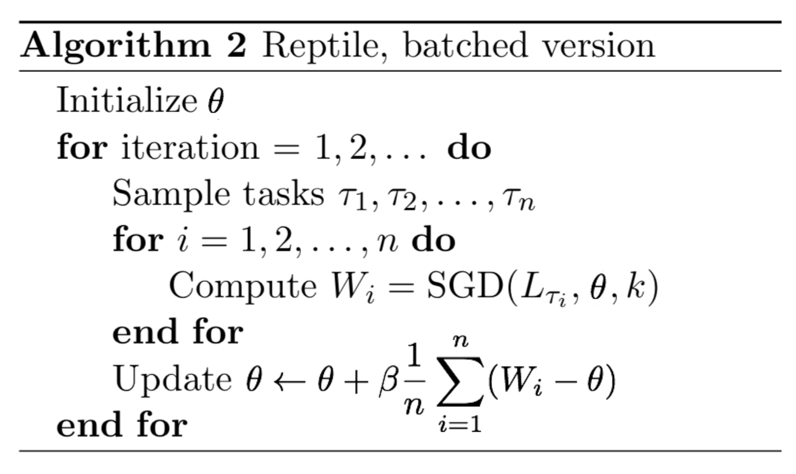
Fig. 13. The batched version of Reptile algorithm. (Image source: original paper)

At a glance, the algorithm looks a lot like an ordinary SGD. However, because the task-specific optimization can take more than one step. it eventually makes $\text{SGD}(\mathbb{E} \tau[\mathcal{L}{\tau}], \theta, k)$ diverge from $\mathbb{E}\tau [\text{SGD}(\mathcal{L}{\tau}, \theta, k)]$ when k > 1.

The Optimization Assumption

Assuming that a task $\tau \sim p(\tau)$ has a manifold of optimal network configuration, $\mathcal{W}_{\tau}^*$. The model $f_\theta$ achieves the best performance for task $\tau$ when $\theta$ lays on the surface of $\mathcal{W}_{\tau}^*$. To find a solution that is good across tasks, we would like to find a parameter close to all the optimal manifolds of all tasks:

$$\theta^* = \arg\min_\theta \mathbb{E}_{\tau \sim p(\tau)} [\frac{1}{2} \text{dist}(\theta, \mathcal{W}_\tau^*)^2]$$

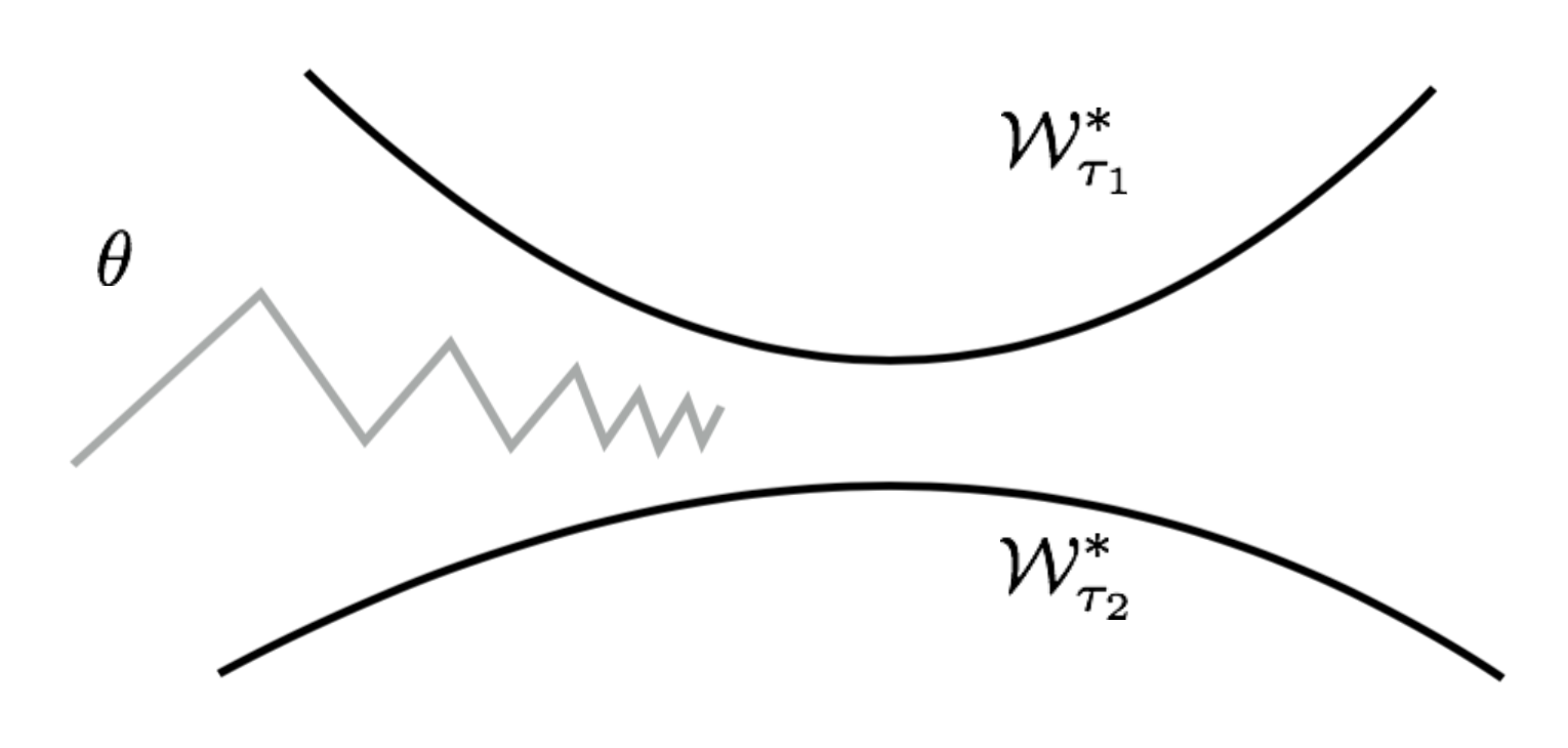
Fig. 14. The Reptile algorithm updates the parameter alternatively to be closer to the optimal manifolds of different tasks. (Image source: original paper)

Let’s use the L2 distance as $\text{dist}(.)$ and the distance between a point $\theta$ and a set $\mathcal{W}_\tau^*$ equals to the distance between $\theta$ and a point $W_{\tau}^*(\theta)$ on the manifold that is closest to $\theta$:

$$\text{dist}(\theta, \mathcal{W}_{\tau}^*) = \text{dist}(\theta, W_{\tau}^*(\theta)) \text{, where }W_{\tau}^*(\theta) = \arg\min_{W\in\mathcal{W}_{\tau}^*} \text{dist}(\theta, W)$$

The gradient of the squared euclidean distance is:

$$\begin{aligned} \nabla_\theta[\frac{1}{2}\text{dist}(\theta, \mathcal{W}_{\tau_i}^*)^2] &= \nabla_\theta[\frac{1}{2}\text{dist}(\theta, W_{\tau_i}^*(\theta))^2] & \\ &= \nabla_\theta[\frac{1}{2}(\theta - W_{\tau_i}^*(\theta))^2] & \\ &= \theta - W_{\tau_i}^*(\theta) & \scriptstyle{\text{; See notes.}} \end{aligned}$$

Notes: According to the Reptile paper, “the gradient of the squared euclidean distance between a point Θ and a set S is the vector 2(Θ − p), where p is the closest point in S to Θ”. Technically the closest point in S is also a function of Θ, but I’m not sure why the gradient does not need to worry about the derivative of p. (Please feel free to leave me a comment or send me an email about this if you have ideas.)

Thus the update rule for one stochastic gradient step is:

$$\theta = \theta - \alpha \nabla_\theta[\frac{1}{2} \text{dist}(\theta, \mathcal{W}_{\tau_i}^*)^2] = \theta - \alpha(\theta - W_{\tau_i}^*(\theta)) = (1-\alpha)\theta + \alpha W_{\tau_i}^*(\theta)$$

The closest point on the optimal task manifold $W_{\tau_i}^*(\theta)$ cannot be computed exactly, but Reptile approximates it using $\text{SGD}(\mathcal{L}_\tau, \theta, k)$.

Reptile vs FOMAML

To demonstrate the deeper connection between Reptile and MAML, let’s expand the update formula with an example performing two gradient steps, k=2 in $\text{SGD}(.)$. Same as defined above, $\mathcal{L}^{(0)}$ and $\mathcal{L}^{(1)}$ are losses using different mini-batches of data. For ease of reading, we adopt two simplified annotations: $g^{(i)}_j = \nabla_{\theta} \mathcal{L}^{(i)}(\theta_j)$ and $H^{(i)}_j = \nabla^2_{\theta} \mathcal{L}^{(i)}(\theta_j)$.

$$\begin{aligned} \theta_0 &= \theta_\text{meta}\\ \theta_1 &= \theta_0 - \alpha\nabla_\theta\mathcal{L}^{(0)}(\theta_0)= \theta_0 - \alpha g^{(0)}_0 \\ \theta_2 &= \theta_1 - \alpha\nabla_\theta\mathcal{L}^{(1)}(\theta_1) = \theta_0 - \alpha g^{(0)}_0 - \alpha g^{(1)}_1 \end{aligned}$$

According to the early section, the gradient of FOMAML is the last inner gradient update result. Therefore, when k=1:

$$\begin{aligned} g_\text{FOMAML} &= \nabla_{\theta_1} \mathcal{L}^{(1)}(\theta_1) = g^{(1)}_1 \\ g_\text{MAML} &= \nabla_{\theta_1} \mathcal{L}^{(1)}(\theta_1) \cdot (I - \alpha\nabla^2_{\theta} \mathcal{L}^{(0)}(\theta_0)) = g^{(1)}_1 - \alpha H^{(0)}_0 g^{(1)}_1 \end{aligned}$$

The Reptile gradient is defined as:

$$g_\text{Reptile} = (\theta_0 - \theta_2) / \alpha = g^{(0)}_0 + g^{(1)}_1$$

Up to now we have:

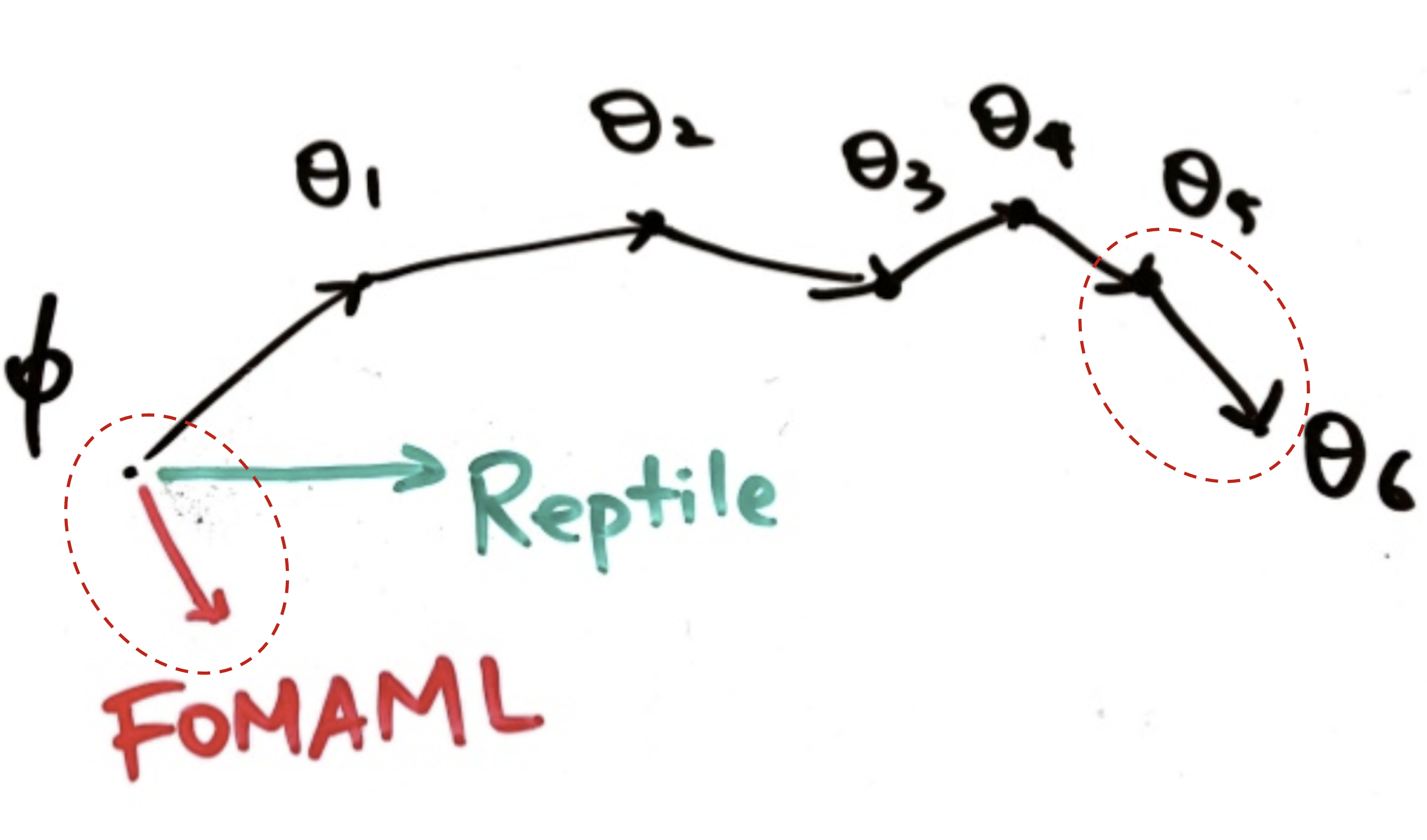
Fig. 15. Reptile versus FOMAML in one loop of meta-optimization. (Image source: slides on Reptile by Yoonho Lee.)

$$\begin{aligned} g_\text{FOMAML} &= g^{(1)}_1 \\ g_\text{MAML} &= g^{(1)}_1 - \alpha H^{(0)}_0 g^{(1)}_1 \\ g_\text{Reptile} &= g^{(0)}_0 + g^{(1)}_1 \end{aligned}$$

Next let’s try further expand $g^{(1)}_1$ using Taylor expansion. Recall that Taylor expansion of a function $f(x)$ that is differentiable at a number $a$ is:

$$f(x) = f(a) + \frac{f'(a)}{1!}(x-a) + \frac{f''(a)}{2!}(x-a)^2 + \dots = \sum_{i=0}^\infty \frac{f^{(i)}(a)}{i!}(x-a)^i$$

We can consider $\nabla_{\theta}\mathcal{L}^{(1)}(.)$ as a function and $\theta_0$ as a value point. The Taylor expansion of $g_1^{(1)}$ at the value point $\theta_0$ is:

$$\begin{aligned} g_1^{(1)} &= \nabla_{\theta}\mathcal{L}^{(1)}(\theta_1) \\ &= \nabla_{\theta}\mathcal{L}^{(1)}(\theta_0) + \nabla^2_\theta\mathcal{L}^{(1)}(\theta_0)(\theta_1 - \theta_0) + \frac{1}{2}\nabla^3_\theta\mathcal{L}^{(1)}(\theta_0)(\theta_1 - \theta_0)^2 + \dots & \\ &= g_0^{(1)} - \alpha H^{(1)}_0 g_0^{(0)} + \frac{\alpha^2}{2}\nabla^3_\theta\mathcal{L}^{(1)}(\theta_0) (g_0^{(0)})^2 + \dots & \scriptstyle{\text{; because }\theta_1-\theta_0=-\alpha g_0^{(0)}} \\ &= g_0^{(1)} - \alpha H^{(1)}_0 g_0^{(0)} + O(\alpha^2) \end{aligned}$$

Plug in the expanded form of $g_1^{(1)}$ into the MAML gradients with one step inner gradient update:

$$\begin{aligned} g_\text{FOMAML} &= g^{(1)}_1 = g_0^{(1)} - \alpha H^{(1)}_0 g_0^{(0)} + O(\alpha^2)\\ g_\text{MAML} &= g^{(1)}_1 - \alpha H^{(0)}_0 g^{(1)}_1 \\ &= g_0^{(1)} - \alpha H^{(1)}_0 g_0^{(0)} + O(\alpha^2) - \alpha H^{(0)}_0 (g_0^{(1)} - \alpha H^{(1)}_0 g_0^{(0)} + O(\alpha^2))\\ &= g_0^{(1)} - \alpha H^{(1)}_0 g_0^{(0)} - \alpha H^{(0)}_0 g_0^{(1)} + \alpha^2 \alpha H^{(0)}_0 H^{(1)}_0 g_0^{(0)} + O(\alpha^2)\\ &= g_0^{(1)} - \alpha H^{(1)}_0 g_0^{(0)} - \alpha H^{(0)}_0 g_0^{(1)} + O(\alpha^2) \end{aligned}$$

The Reptile gradient becomes:

$$\begin{aligned} g_\text{Reptile} &= g^{(0)}_0 + g^{(1)}_1 \\ &= g^{(0)}_0 + g_0^{(1)} - \alpha H^{(1)}_0 g_0^{(0)} + O(\alpha^2) \end{aligned}$$

So far we have the formula of three types of gradients:

$$\begin{aligned} g_\text{FOMAML} &= g_0^{(1)} - \alpha H^{(1)}_0 g_0^{(0)} + O(\alpha^2)\\ g_\text{MAML} &= g_0^{(1)} - \alpha H^{(1)}_0 g_0^{(0)} - \alpha H^{(0)}_0 g_0^{(1)} + O(\alpha^2)\\ g_\text{Reptile} &= g^{(0)}_0 + g_0^{(1)} - \alpha H^{(1)}_0 g_0^{(0)} + O(\alpha^2) \end{aligned}$$

During training, we often average over multiple data batches. In our example, the mini batches (0) and (1) are interchangeable since both are drawn at random. The expectation $\mathbb{E}_{\tau,0,1}$ is averaged over two data batches, ids (0) and (1), for task $\tau$.

Let,

• $A = \mathbb{E}_{\tau,0,1} [g_0^{(0)}] = \mathbb{E}_{\tau,0,1} [g_0^{(1)}]$; it is the average gradient of task loss. We expect to improve the model parameter to achieve better task performance by following this direction pointed by $A$.
• $B = \mathbb{E}_{\tau,0,1} [H^{(1)}_0 g_0^{(0)}] = \frac{1}{2}\mathbb{E}_{\tau,0,1} [H^{(1)}_0 g_0^{(0)} + H^{(0)}_0 g_0^{(1)}] = \frac{1}{2}\mathbb{E}_{\tau,0,1} [\nabla_\theta(g^{(0)}_0 g_0^{(1)})]$; it is the direction (gradient) that increases the inner product of gradients of two different mini batches for the same task. We expect to improve the model parameter to achieve better generalization over different data by following this direction pointed by $B$.

To conclude, both MAML and Reptile aim to optimize for the same goal, better task performance (guided by A) and better generalization (guided by B), when the gradient update is approximated by first three leading terms.

$$\begin{aligned} \mathbb{E}_{\tau,1,2}[g_\text{FOMAML}] &= A - \alpha B + O(\alpha^2)\\ \mathbb{E}_{\tau,1,2}[g_\text{MAML}] &= A - 2\alpha B + O(\alpha^2)\\ \mathbb{E}_{\tau,1,2}[g_\text{Reptile}] &= 2A - \alpha B + O(\alpha^2) \end{aligned}$$

It is not clear to me whether the ignored term $O(\alpha^2)$ might play a big impact on the parameter learning. But given that FOMAML is able to obtain a similar performance as the full version of MAML, it might be safe to say higher-level derivatives would not be critical during gradient descent update.